Team:Cambridge-JIC/Autofocus
The Solution
The strategy of the autofocus algorithm is to calculate the focus score for each frame imaged while gradually changing the sample-objective distance. The most sharply focused image corresponds to the maximised focus score. The physics behind the process is very simple: the image of an object, viewed through a lens, is produced at a particular distance from the lens. At any shorter/longer distance from the lens, the light rays from a single point on the object do not converge into a point, causing the image to be blurred. The focus score can be simply regarded as a mathematical function with a single maximum.
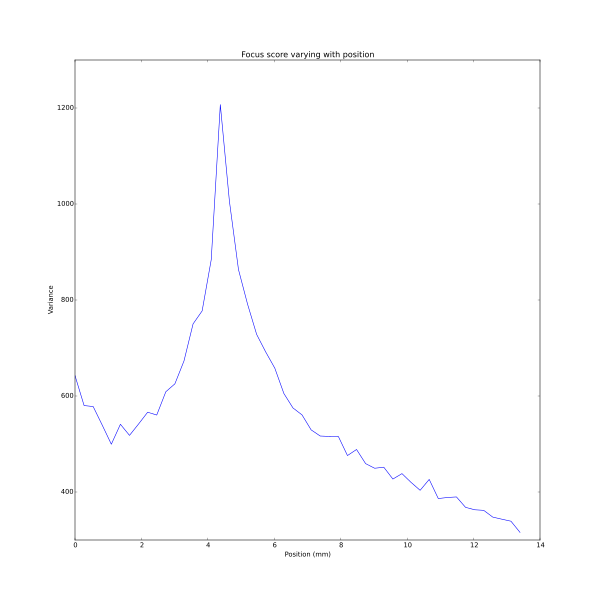
Fig, 1: The plot shows the focus score of an image as a function of the distance between the objective and the sample: it is clear that the function has a single maximum. The corresponding images recorded at these distances are also shown. Note that most of the time during the search, the sample remains significantly out-of-focus.
There are, however, several issues to consider and multiple methods exist for calculating the focus score. In addition, there are many ways to scan around for the best focus score. The challenge was to find the most robust solutions. Below is an outline of the development process:
Tested out focus scores based on variance, as this was recommended by both sources [1][2] on artificially blurred out images (Gaussian blur with different standard deviations). This worked well. Variance was chosen as the focus measure to implement since it is quick to evaluate (speed being an important priority), and numpy (a Python library) has a function that does this already.
Implemented an autofocus method for multi-resolution search (described in source [2], section 16.3.3).
Implemented DWT (Discrete Wavelet Transform) to decompose image to low resolution versions. This was expected to allow for faster computation and autofocusing. In practice, there was no significant computational advantage to this, so low-res images were not used in the final algorithm.
Having been able to determine a focus score for an image, the next step was to develop methods for finding the most in-focus position. This involves several important issues:
Delays from moving the motor to receiving an updated frame - this is a common issue with feedback loops, everywhere from biological systems to adjusting the temperature of the shower. Failure to deal with this can result in oscillations around the set point, with the image remaining just out of focus most of the time. We dealt with this by introducing a delay between sending a "move motor" command and a "read focus score" command to attempt to match the two. Reading a focus score when the motors were no longer moving is not an issue, but reading a value before the desired position has been reached is. Thus, it is beneficial to err on the side of an increased counter-delay, though at the expense of the time for autofocus to take place.
Unreliability of motor positioning - when moving +400 steps and then -400 steps, there is no guarantee of returning to exactly the same position.
Local maxima not being the global maxima - A more theoretical issue than the practical ones above. Once reaching an area of high focus value, there is little guarantee that this is the most focused plane in the image. This is in contrast to the issue above - if we "give up" an area of high focus, we may find it difficult to retrieve it. We ignored this issue in favour of the more practical ones above - attempting to account for global maxima of focus scores would require the autofocus procedure to be far longer than desirable. We also implemented a naive dynamic threshold to stop moving the z axis once the focus was "good enough", a value for which is empirically derived.
We settled for a hill-climbing approach. Imagining the theoretical focus score for all possible z values on a graph may look like a hill. This algorithm attempts to "climb" that hill of focus scores. This algorithm assesses the focus scores of individual frames, moving in the direction where the focus is increasing. If the focus decreases, the motors are reversed in smaller increments. This process is repeated several times until an exit condition is reached.
We tried a variety of other approaches to tackle these issues:
Implemented the Gaussian approximation to predict in-focus position from the interval. This assumes that the image is formed from paraxial rays only, which is a good approximation in the case of microscopic imaging.
Implemented the Fibonacci search algorithm. It turns out that this is the optimal search algorithm for the situation of unimodal functions [2].
Implemented the parabola approximation to find in focus position.
Gradient search, which is a simple technique to locate local extrema, was also attempted but did not give satisfactory results, as the learning rate required for convergence was slow. Also, noise from images drastically disrupted the calculations. This was a significant problem even when the gradient was calculated by taking multiple pictures around the point of interest.
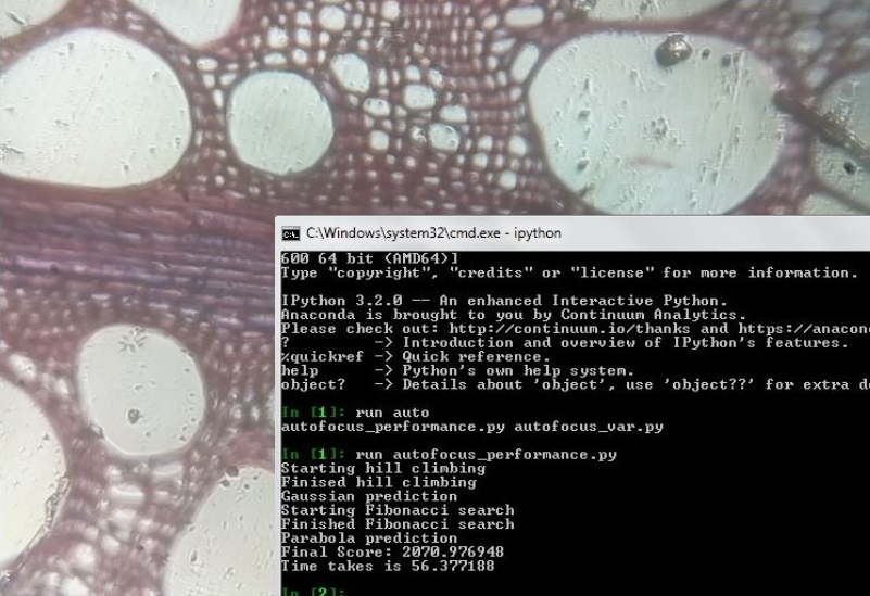
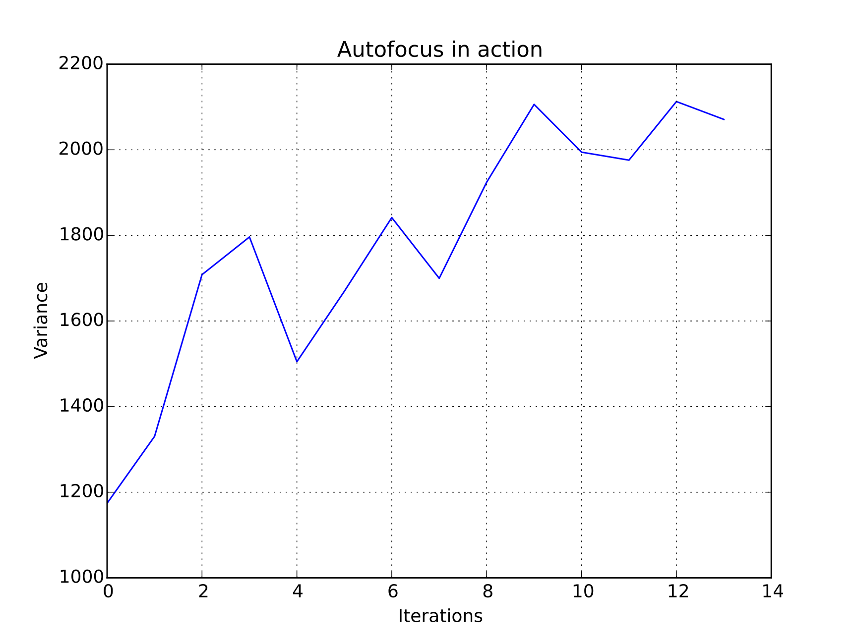
Fig. 2: Autofocus algorithm in action: the plot shows the increase of the variance (i.e. the focus score) of the image with each iteration.

Fig. 3: Indicative proportion of time spent in each phase of one implementation of an autofocus search
The performance of the final autofocus algorithm varies, depending on the starting point of the search. A typical processing time is around 5s, which allows for autofocus during live-stream imaging through the Webshell.
The autofocus algorithm we have implemented is open for further improvements and performance enhancement. Ideas for future development include:
A better hill climbing algorithm for finer focus after reaching the "almost focused stage"
Automatic measurement of the actual height to the CCD
More reliable motors use to improve precision
The Autofocus algorithm we have developed can be found in the Downloads page. The whole Software team contributed to its development.
References:
[1] Firestone, L., Cook, K., Culp, K., Talsania, N. and Preston, K. (1991). Comparison of autofocus methods for automated microscopy. Cytometry, 12(3), pp.195-206
[2] Wu, Q., Merchant, F. and Castleman, K. (2008). Microscope image processing. Amsterdam: Elsevier/Academic Press.