Team:Oxford/Modeling

Modelling

Introduction

Mathematical modelling plays a crucial role in Synthetic Biology by acting as a link between the conception and the physical realisation of a biological circuit. Our modelling team has evaluated the effectiveness of initial designs, and has provided insight into how the system can (or must) be improved.

Our team experimentally validated that Escherichia coli can secrete enzymes which break down the biofilms associated with urinary infections. However, it is difficult to directly measure whether our enzymes are produced in a sufficient quantity to be a more effective treatment than antibiotics. We measured gene expression and diffusion of widely-used chemicals, and then used our model to estimate the number of E. coli cells that would make our project a more effective treatment than antibiotics. We expect to have to improve our system to make it realistic.

To help readers of all kinds and specialisations understand this page we have produced guides for all the modelling techniques used in this section. They are available in our Modelling Tutorial page and will be linked to when appropriate.

Gene expression rates

In this section we look at our cells in isolation in order to assess their functionality and answer important questions such as “how long does it take to produce a certain concentration of product?” The end result - the final concentration of useful enzyme that is produced in the cell - is required for our diffusion model.

Arabinose-induced expression

We have decided to use an arabinose-induced promoter for the expression of a number of our proteins. This promoter can be modelled as the following chemical system:

\[(Arab:AraC)\overset{K}{\rightarrow}mRNA\overset{\alpha}{\rightarrow}P\] \[mRNA\overset{\gamma_{1}}{\rightarrow}\phi\quad P\overset{\gamma_{2}}{\rightarrow}\phi\]

Our promoter, pBAD, binds to AraC and this represses transcription of mRNA. Arabinose will bind to AraC and form the Arab:AraC compound, allowing transcription to occur.

For this system we will assume that AraC is always in large concentration and that its binding to arabinose happens on a faster time scale to transcription. Therefore, we do not need to consider the individual concentrations of arabinose and AraC, instead we just need to include the concentration of the complex (Arab:AraC). The rate \(K\) is not just a simple constant and is given as the Hill function in the equations below.

Using Michaelis-Mentin kinetics, we arrive at the equations:

\[\dfrac{d[mRNA]}{dt}=K_{max}\dfrac{[Arab:AraC]^{n}}{K_{half}^{n}+[Arab:AraC]^{n}}-\gamma_{1}[mRNA]\] \[\dfrac{d\left[P\right]}{dt}=\alpha\left[mRNA\right]-\gamma_{2}\left[P\right]\]

Where \([Arab]\), \([AraC]\), \([Arab:AraC]\), \([mRNA]\) and \([P]\) represent the concentrations of arabinose, AraC, Arab:AraC, mRNA and our product protein respectively. We define the remaining symbols in the table below.

Symbol	Definition	Initial Value/Literature Value	Fitted
\(\alpha\)	Translation rate	\(15ntd\: s^{-1}\)/length of sequence [6]	\(6.6ntd\: s^{-1}\)/length of sequence
\(\gamma_{1}\)	Combined degradation and dilution rate of mRNA	\(2.2\times10^{-3}s^{-1}\) [5, 10]	\(1.1\times10^{-2}s^{-1}\)
\(\gamma_{2}\)	Combined degradation and dilution rate of GFP	\(5.2\times10^{-4}s^{-1}\) [5, 11]	\(1.1\times10^{-2}s^{-1}\)
\(K_{max}\)	Maximal transcription rate	\(50ntd\: s^{-1}\)/length of sequence [6]	\(47ntd\: s^{-1}\)/length of sequence
\(K_{half}\)	Half-maximal transcription rate	\(160\mu M\) [7]	\(100\mu M\)
\(n\)	Hill coefficient	\(2.65\) [8]	\(2.73\)

This table contains literature values for the parameters, found from a number of sources. We then measured GFP expression in E. coli to extract experimental values. Here is a plot showing the fit of this model to our experimental data.

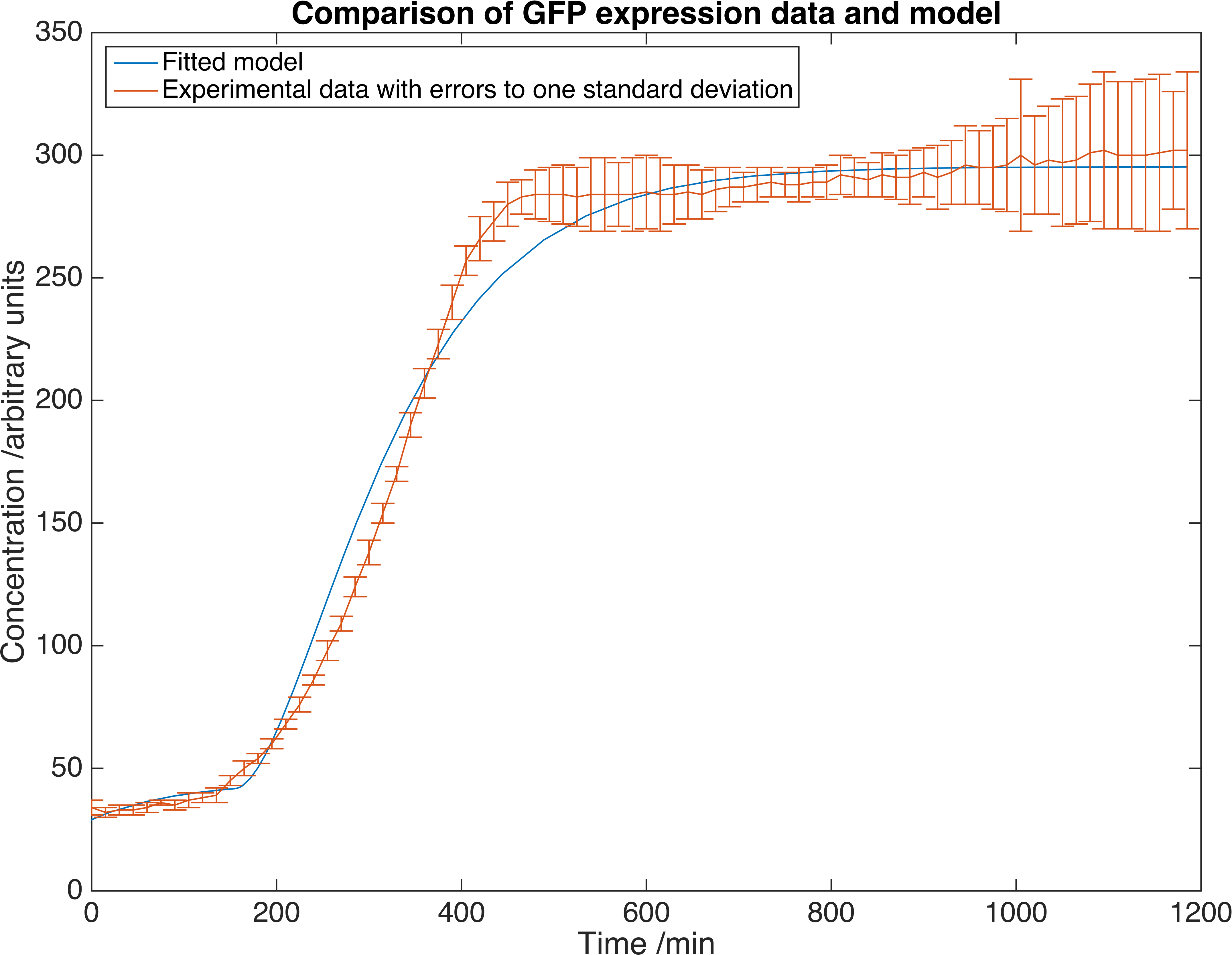
Results showing GFP concentration as a function of time, matched to our deterministic model. Errors are given to one standard deviation and an arbitrary scaling factor is included as a fitted parameter.

We can now calculate the limiting concentrations that our products will be expressed. The dilution rate and Hill coefficient of our cells is the same for GFP and our proteins, but the transcription and translation rates are dependent on the sequence length of the protein. Here is a table showing the relevant proteins and sequence lengths:

Product	Sequence Length (/bp)
pBAD HisB DNase DsbA	621
pBAD HisB MccS	414
pBAD HisB Art-175 DsbA	987
pBAD HisB Art-175 YebF	1284
pBAD HisB Art-E	632
pBAD HisB Art-175 Fla	1095
pBAD HisB Art-175	936
pBAD HisB DNase	570

We now can run our model of the system by solving the set of equations using the MATLAB ordinary differential equation solver ode15s. Below is a plot of the concentration of product against time for each protein expressed with this inducer-promoter pair where the expression is induced by a step function:

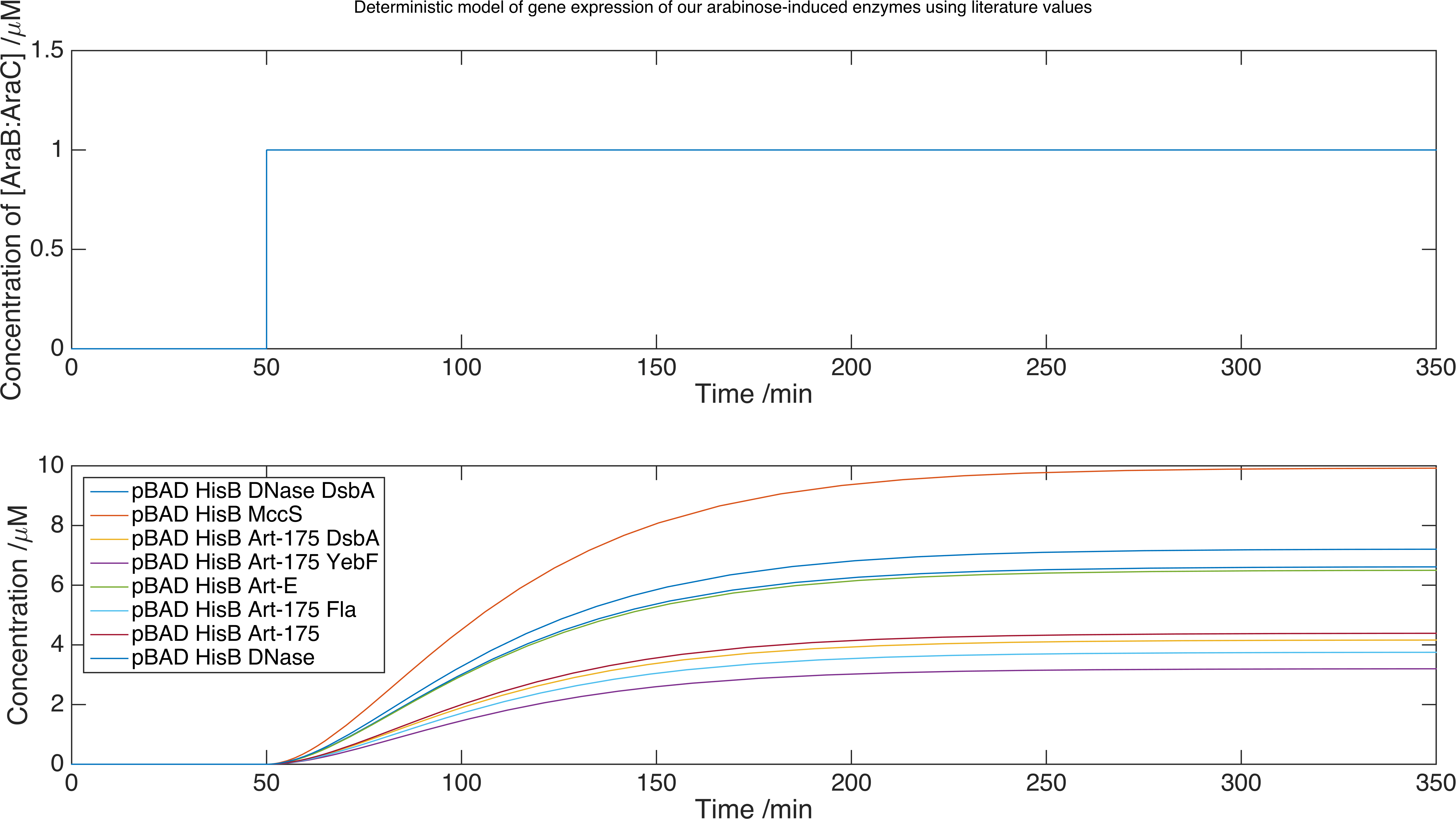
Model data for each of the enzymes we plan to release, using the parameters we found from our experimental data. We found our limiting concentrations were of order \(\mu M\).

The advantage of this method is that we have not had to directly measure expression data for all of our enzymes, which is a difficult process. We conclude that we should obtain enzyme expression of order \(\mu M\) within 350 minutes. However, the scaling factor we introduced in our fitting function is no substitute for a calibration curve to match GFP fluorescence with GFP concentration. For this reason, we conservatively estimate that our proteins are expressed at \(nM\) concentration.

Delivery

With the information about the rates of production and concentrations of our products, we can look at how the products behave once they leave the cell. Our enzymes are first secreted from the cells, and then out of our containment beads to the biofilms they target. We can provide an estimate of the time scale that our project is working on and assess any need for optimisation of enzyme efficiency.

Dispersin B

Dispersin B is one of the anti-biofilm agents we are using in our project and will be the focus of this delivery section. As such we will assume that conclusions reached apply to all of our enzymes.

A concentration of Dispersin B of 60μg/ml is required to destroy a biofilm that has already formed on a surface [1]. This equates to a concentration of 1.5μM. This is higher than the steady-state gene expression concentration we can expect from our cells, meaning that our system cannot rely solely on diffusion to transport our enzymes to the biofilm. We will therefore model these diffusion systems assuming that our cells are expressing at a 2μM concentration and later we will look at optimising the gene expression to this level.

Beads

Diffusion

The bead delivery system consists of our cells being contained in alginate spheres. Water is passed through a container filled with the beads allowing our enzymes to diffuse from the alginate to where they are required. More details about the design of the system can be found here. Below is a diagram of our cells secreting proteins out of the beads that they are contained in.

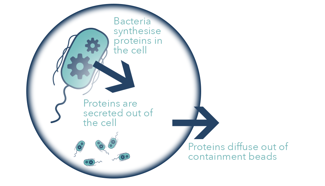
Diagram of secretion through our containment beads.

To determine the convection mass transfer coefficient of Dispersin B from our gel spheres we looked at the diffusion data obtained from this experiment involving the diffusion of crystal violet from our beads. By analysing the system we can produce a theoretical formula for the concentration of crystal violet in the bulk water as a function of time:

\[c_{f}=\dfrac{c_{bo}}{1+\frac{V_{f}}{V_{b}}}\left(1-\exp\left(\dfrac{-K_{m}A_{b}\left(1+\frac{V_{f}}{V_{b}}\right)t}{V_{f}}\right)\right)\]

Symbol	Definition	Value	Units
\(A_{b}\)	Total surface area of the beads	\(0.024\)	\(m^{2}\)
\(V_{b}\)	Total volume of beads	\(1.4\times10^{-5}\)	\(m^{3}\)
\(c_{bo}\)	Initial dye concentration in beads	\(0.025\)	\(M\)
\(V_{f}\)	Volume of fluid surrounding the beads	\(V_{f}=V_{fo}-\dfrac{1\times10^{-6}}{10}t\)	\(m^{3}\)
\(V_{fo}\)	Initial volume of fluid surrounding the beads	\(1\times10^{-4}\)	\(m^{3}\)
\(t\)	Time	\(-\)	\(min\)
\(c_{f}\)	Concentration of fluid surrounding beads	\(-\)	\(M\)
\(K_{m}\)	Convection mass transfer coefficient	To be fitted	\(mmin^{-1}\)

The volume of fluid is also a function of time in order to account for the removal of 1ml of water every 10 minutes. The area and volume of the beads is equal to that of 660 spheres with diameter 3.39mm.

However, the number of beads is an estimate. Because of this, in order to fit the curve to the experimental data we must scale the experimental data by an unknown factor. Therefore we pre-multiply our equation with an arbitrary scaling factor which, along with the convection diffusion coefficient - \(K_{m}\) - is determined by our fitting function.

By fitting the model to our data we returned the value of \(K_{m} = 1.7265\times 10^{-5} mmin^{-1}\).

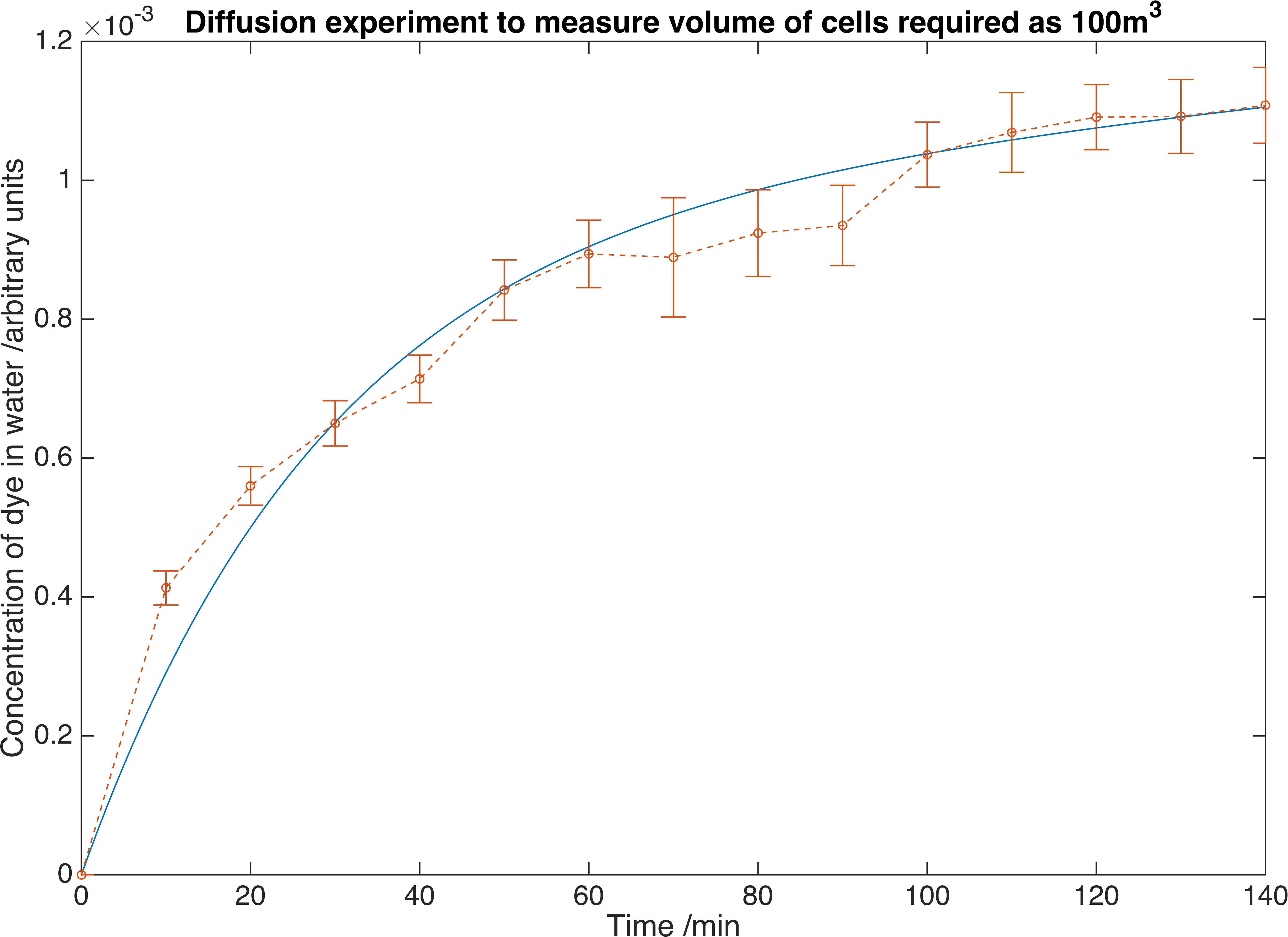
We measure the concentration of crystal violet dye as it diffuses out of our containment beads. Errors are given to one standard deviation and data is fitted to a deterministic model to find the convection mass transfer co-efficient. From this we can determine we would require \(100m^{3}\) of beads to reach the required concentration of our own enzymes.

Dispersin B is a significantly larger molecule than crystal violet so this diffusion coefficient will not be close to that for Dispersin B. To account for this, we estimated the convective mass transfer coefficient \(K_{m}\) for Dispersin B using that obtained for crystal violet by assuming that \(K_{m}\) is proportional to the diffusion constant in water D.

\[\left(K_{m}\right)_{DispersinB} = \dfrac{D_{DispersinB}}{D_{crystal violet}}\left(K_{m}\right)_{crystal violet} \]

Symbol	Definition	Value	Units
\(D_{crystal violet}\)	Mass diffusivity of crystal violet in water	\(2.87\times10^{9}\)[2]	\(\mu m^{2}s^{-1}\)
\(D_{Dispersin B}\)	Mass diffusivity of Dispersin B in water	\(100\) [3]	\(\mu m^{2}s^{-1}\)

By substituting in these values we arrive at \(\left(K_{m}\right)_{DispersinB} = 6.03\times10^{-13} mmin^{-1}\)

Mass Exchange

This result allows us to theorise a mass exchange system. As a first estimate we will assume that the flow through the beads is sufficiently slow to use the convection diffusion coefficient found above. It is also assumed that the gene expression happens on a faster time scale than the diffusion from the beads to the water, enabling us to assume the concentration of enzyme in the beads remains constant. This is supported by our gene expression models. We can now visualize how the concentrations of the fluid will vary with distance along the mass exchanger:

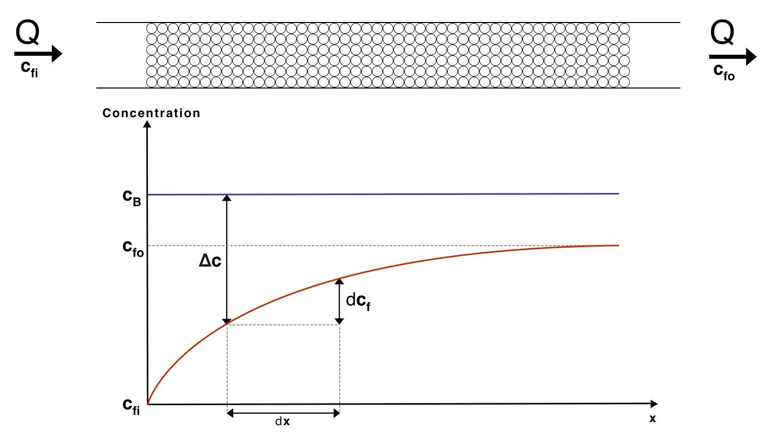
Visualisation of the concentrations of the fluid and the beads along our mass exchanger

The overall system can now be described with the equation:

\[J = K_mA\dfrac{c_{fo}-c_{fi}}{\ln\left(\dfrac{c_{B}-c_{fi}}{c_{B}-c_{fo}}\right)}\]

Therefore

\[A = J\dfrac{\ln\left(\dfrac{c_{B}-c_{fi}}{c_{B}-c_{fo}}\right)}{K_{m}\left(c_{fo}-c_{fi}\right)}\]

Where \(J=Q\left(c_{fo}-c_{fi}\right)\) and \(Q\) is the volume flow rate of water. We have chosen a flow rate range of 10-100ml/min as this is accepted as a safe artificial bladder fill rate [4]. This range results in the following number of beads required to reach the desired concentration:

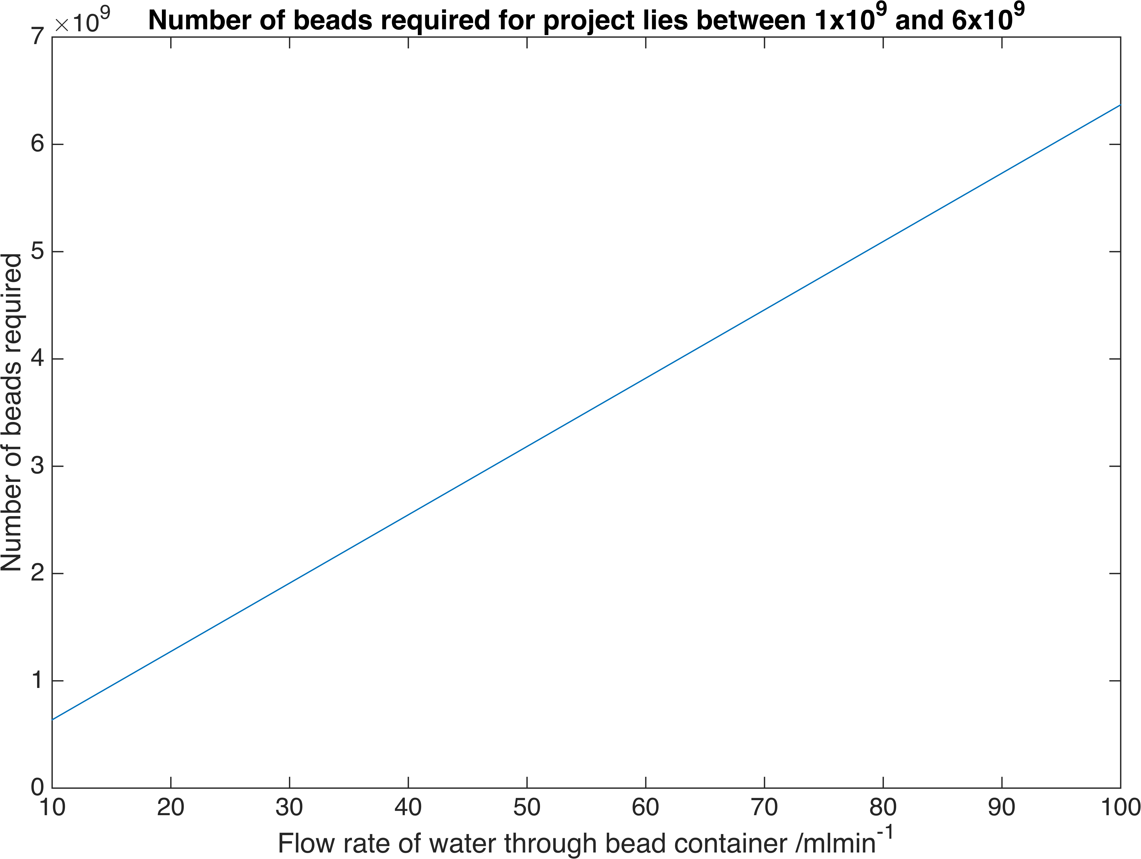
Relationship between the number of bacteria-containment beads required to reach a particular flow rate of our enzymes. These are the flow rates we require for practical use.

Therefore a volume of between \(20.3-203m^3\) of beads is required, assuming a packing efficiency of 64% [9].

This estimation relied upon the flow of fluid around the beads being sufficiently slow such that it may be approximated as stationary, so that mass transfer occurs as natural convection. However, because of the (likely) large volume of beads compared to the cross-sectional area of the catheter, this flow of fluid may have a non-negligable velocity.

Conclusion

Using gene expression and diffusion models, we estimated that we would need around \(100m^3\) of beads to deliver enough enzymes to clear a urinary-infection-associated biofilm. Our treatment will only be more effective than antibiotics if we make our enzymes many orders of magnitude more efficient. This led us to consider an alternative design.

• Introduction
• Gene expression rates
  • Arabinose-induced promoter
• Delivery
  • Dispersin B
  • Beads
    • Diffusion
    • Mass Exchanger
  Conclusion
• References

Made with love by Oxford iGEM

References

- Jeffrey B. Kaplan; Dispersin B polypeptides and uses thereof. Patent PI 8580551, Nov 12, 2013
- http://physicalpharmacy2013.blogspot.co.uk/2013/05/practical-4.html
- "Physical Biology of the Cell", Rob Phillips, Jane Kondev and Julie Theriot (2009). Page 110
- Kim S-Y, Ko SH, Shin MJ, et al. Phasic Changes in Bladder Compliance During Filling Cystometry of the Neurogenic Bladder. Annals of Rehabilitation Medicine. 2014;38(3):342-346. doi:10.5535/arm.2014.38.3.342.
- Liang ST, Ehrenberg M, Dennis P, Bremer H. Decay of rplN and lacZ mRNA in Escherichia coli. J Mol Biol. 1999 May 14 288(4):521-38. p.524 right column bottom paragraph
- Proshkin S, Rahmouni AR, Mironov A, Nudler E. Cooperation between translating ribosomes and RNA polymerase in transcription elongation. Science. 2010 Apr 23 328(5977):504-8. p.505 table 1
- Sourjik V, Berg HC. Functional interactions between receptors in bacterial chemotaxis. Nature. 2004 Mar 25 428(6981):437-41.p.439 left column top paragraph
- Salto R, Delgado A, Michán C, Marqués S, Ramos JL. Modulation of the function of the signal receptor domain of XylR, a member of a family of prokaryotic enhancer-like positive regulators. J Bacteriol. 1998 Feb180(3):600-4. p.601 right column
- S. Torquato, T. M. Truskett, and P. G. Debenedetti Is Random Close Packing of Spheres Well Defined? 2000 Phys. Rev. Lett. 84, 2064
- Selinger DW, Saxena RM, Cheung KJ, Church GM, Rosenow C. Global RNA half-life analysis in Escherichia coli reveals positional patterns of transcript degradation. Genome Res. 2003 Feb13(2):216-23. p.217 left column 2nd paragraph
- Andersen JB, Sternberg C, Poulsen LK, Bjorn SP, Givskov M, Molin S. New Unstable Variants of Green Fluorescent Protein for Studies of Transient Gene Expression in Bacteria. Appl Environ Microbiol. 1998 Jun64(6):2240-6.