Modeling

Bridging length scales and timescales

Overview

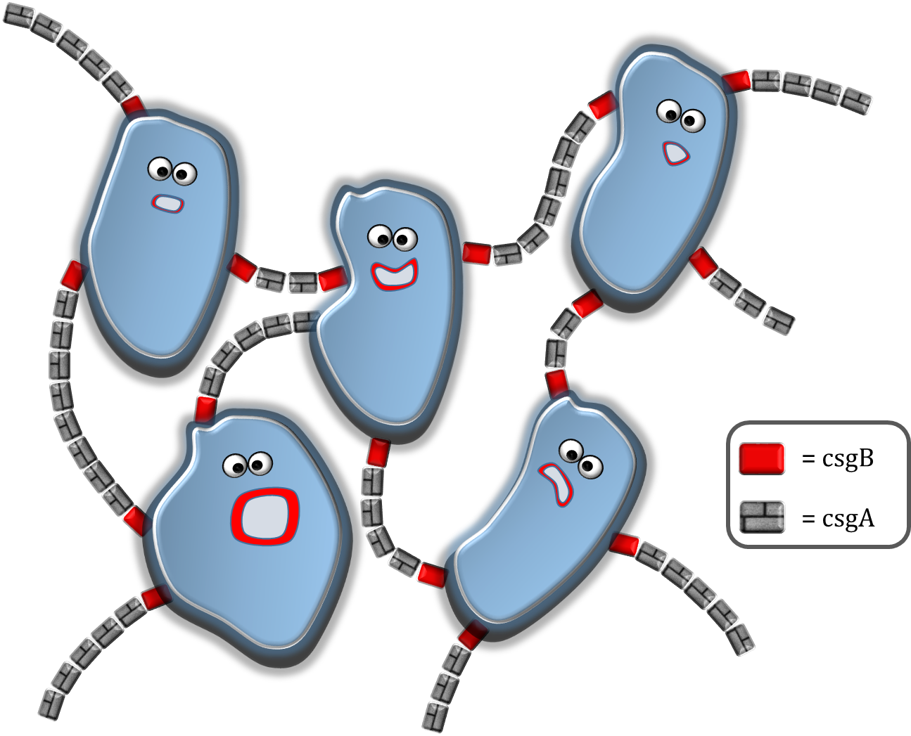
Our main goal is to make a reproducible 3D printed biofilm. The strength of the biofilm is determined by the degree of intercellular connectivity through curli fibers. With modeling, it is possible to determine which factors have a strong influence on the intercellular connectivity. For instance, one could argue that a higher csgB nucleator production would lead to more curli fibers and therefore an improved connectivity. But if the csgA production would be limiting, solely short curli chains would be formed possibly preventing the cells to even interconnect.

Generic placeholder image — **Fig. 1**: Illustration depicting the cells interconnecting by curli fibers. The csgA protein is secreted by the cells to the extracellular space. A curli can be formed when the csgA reacts with the nucleator protein csgB, located at the outer membrane of the cells.

The modeling can be divided in 4 sections. In section 1, the csgA production rate, intracellular csgA concentration and csgB membrane concentration are determined. As our csgA production is controlled under the induction of rhamnose, all rates and concentrations are calculated for two levels of induction [ 0.2% (w/v) and 0.5% (w/v) rhamnose ]. In section 2, the rates and concentrations are used in a grid model which is able to make an estimate on the characteristic time of curli formation. In section 3 the characteristic time for curli formation is used to predict the strength of the formed biofilm.

Finally, in section 4, an application in MATLAB is presented able to calculate the printing time of a certain figure or shape produced with our Biolinker 3D printer. To go to either of these sections, click on one of the buttons below or select your section of interest in the modeling submenu!

Kinetic Modeling

With an inducible promoter, it is possible to have control over the production of your target protein. For us, this protein is csgA under the induction of rhamnose. In the kinetic modeling section, a quantitative model was developed to calculate the promoter strength for different rhamnose induction levels. After determining the intracellular csgA concentration, csgA production rates of 2 and 3 molecules were found for 0.2% (w/v) and 0.5% (w/v) rhamnose induction respectively.

csgA production rate

The csgA production rate is defined as the production of csgA per second per cell. To be able to calculate this number, the following unknown parameters need to be characterized:

I. Activity of the promoter (with different levels of rhamnose induction).

II. Export rate of csgA to the extracellular space.

If these parameters are known, a model for the csgA production can be formulated and the export of csgA to the extracellular space can be calculated.

The activity of the promoter, denoted as PoPs, can be calculated by a kinetic experiment with GFP. For this experiment, we made a construct with GFPmut3 (modified GFP variant with stronger fluorescent signal) and csgA under the same rhamnose promoter. The constructs used for this experiment are depicted in Fig. 2.

As csgA and GFP are under the same promoter, the fluorescence signal of GFP can be related to the production of csgA. It is assumed that the promoter activity is independent of the addition of the GFPmut3 gene.

As already mentioned in the “Project” section, both the fluorescence and OD600 were measured. It is important to also measure the cell density, as we are interested in the fluorescence per cell per second. To calculate how much fluorescence corresponds to a certain amount of GFP (in nanogram), a calibration curve has been constructed with wtGFP. As the ratio of emission maxima for GFPmut3 relative to wtGFP is 21 at an excitation of 488nm (Brendan et. al), the correct mass amount of GFP mut3 could be determined.

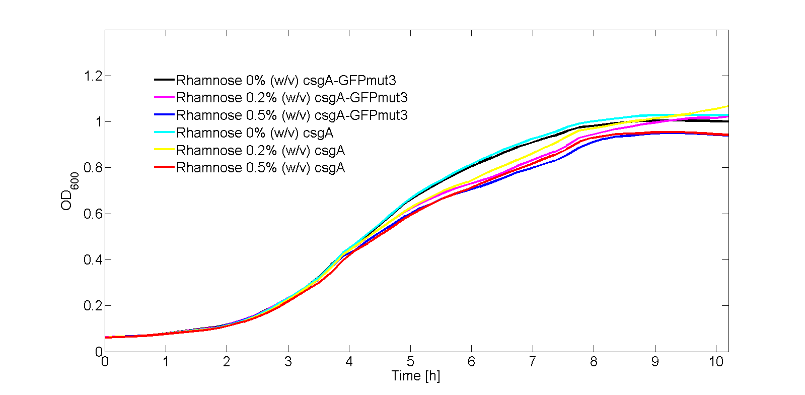
In Fig. 3, the OD600 is plotted for each of the samples in the kinetic experiment. As can be seen from Fig. 3, there is some difference in OD600 between the samples. Therefore, the fluorescence signal normalized by the number of cells as shown in Fig. 4:

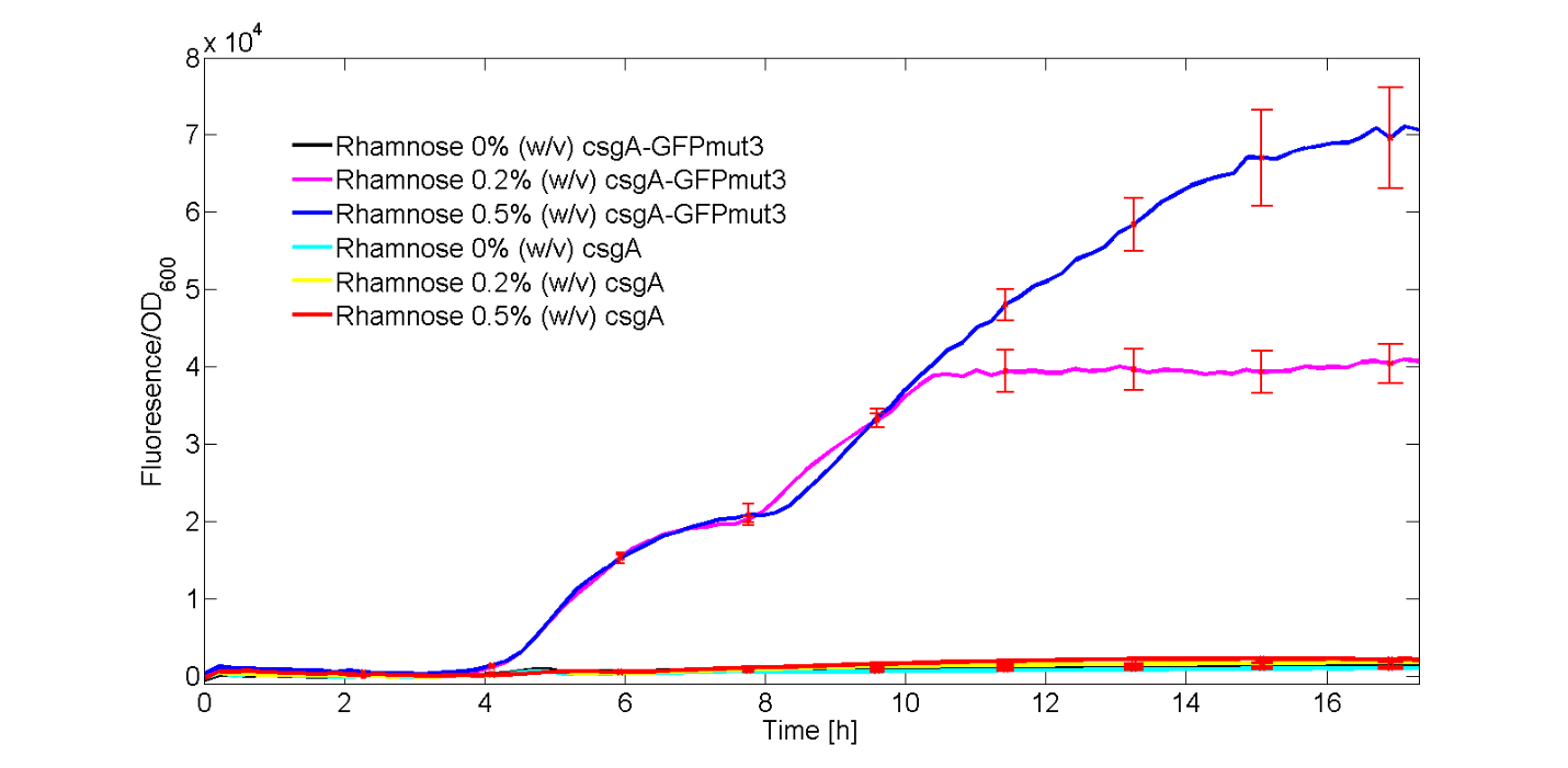
As can be seen from Fig. 4, GFPmut3 only appears if the culture has been induced by rhamnose. Furthermore, it can be seen that a higher induction level of rhamnose leads to an increase in GFPmut3 and thus fluorescence. Finally, as the fluorescence signal is normalized by the cell density, one can make statements about the activity of the rhamnose promoter. The promoter seems to not be active right after induction, but more after 3 or 4 hours. This is in accordance with data from literature (Wegerer et. al), in which a low amount of fluorescence with a rhamnose promoter was observed after 2 hours of induction.

The calibration line of fluorescence versus mass amount GFPmut3 is given in Fig. 5.

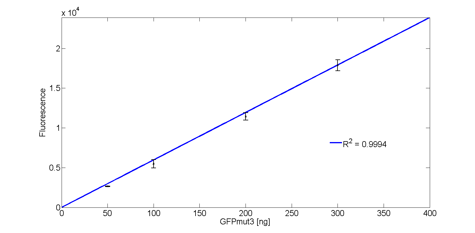
The corresponding function of the GFPmut3 calibration line with mass_GFP in nanogram is:

With the calibration line, which was made with the exact same settings as the kinetic experiment, the mass amount of GFPmut3 per cell can be calculated. With Eq. 1, the fluorescence signal was converted to mass amount of GFPmut3 for rhamnose induction of 0.2% (w/v) and 0.5% (w/v).

After this conversion, the units are still in nanogram per OD600. As the desired unit is molecules per cells, the following dimension analysis has been performed:

The result of this unit conversion is shown in Fig. 6:

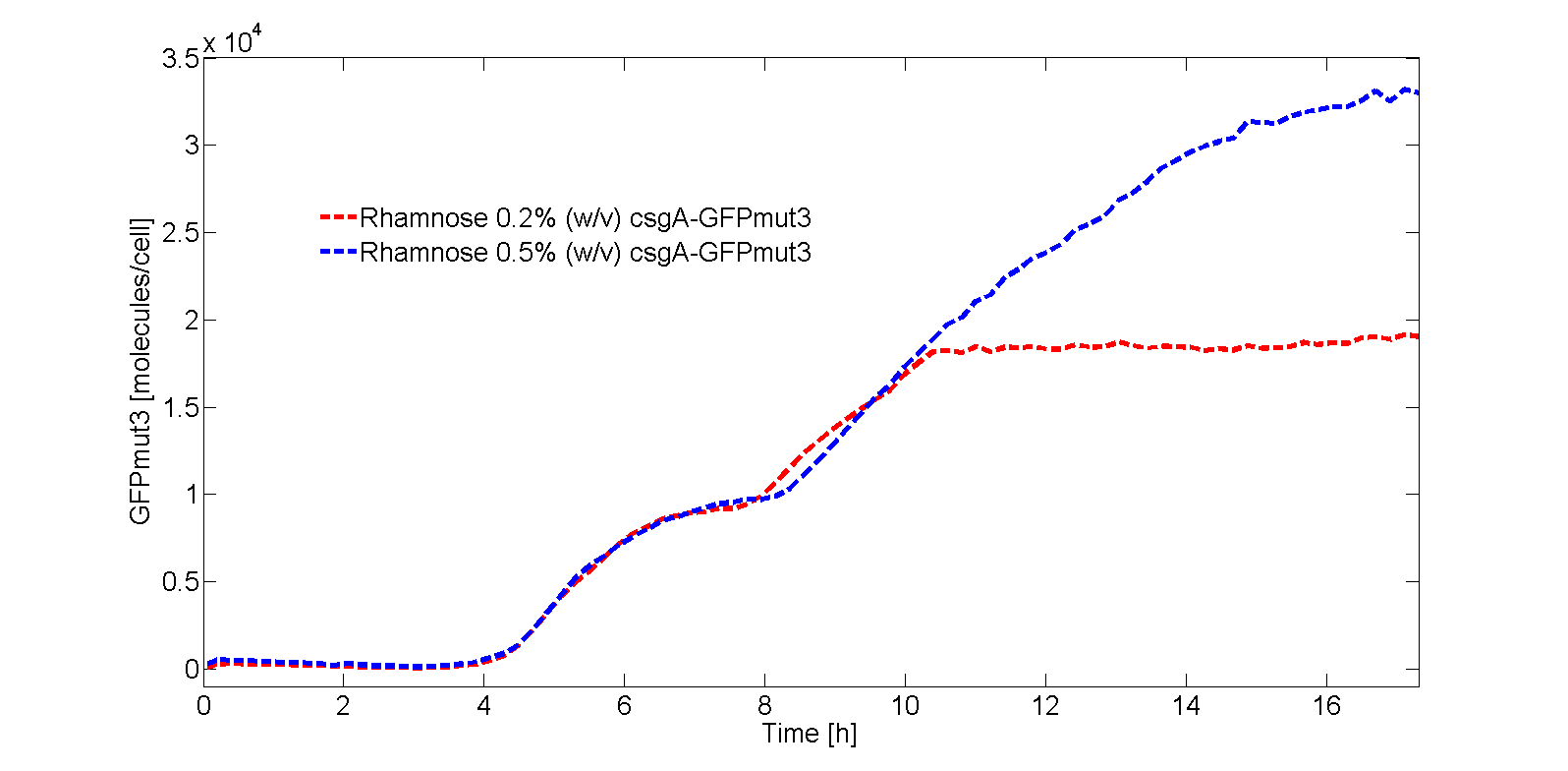
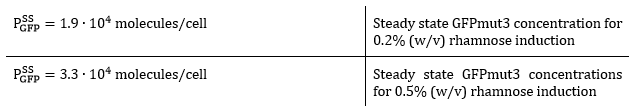
The GFPmut3 steady state concentrations are thus:

As the data is now converted to molecules per cell, it is possible to construct a model with the purpose of predicting the same steady state levels as in the performed experiments. The only unknown remaining in this model is the promoter activity, which can be varied to correctly fit the data.

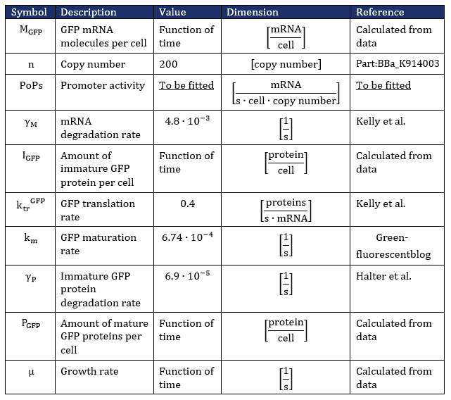
The model that was made is a mathematical model of ordinary differential equations (ODE’s) describing the GFP mRNA concentration (Eq. 2), immature GFP protein concentration (Eq. 3) and mature GFP protein concentration (Eq. 4) in Table 1. All concentrations are modeled per cell per second. The immature protein is the nonfluorescent GFP, the mature protein is the fluorescent protein (which will be fitted to the data).

In the kinetic model, the growth rate of the bacteria is not a constant (as can be seen from Fig. 3). The bacteria grow exponentially from 2 to 3. 5 hours before going into the stationary phase. Until 2 hours, the bacteria are in the lag phase of growth. This growing behavior, in the order lag phase - exponential phase - stationary phase, is characterized with the following differential equation (Koseki et al.):

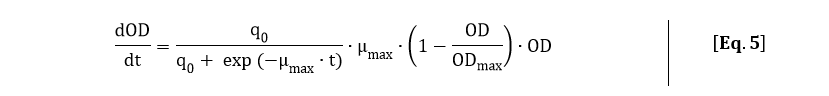
In order to fit Eq. 5 to the OD600 data depicted in Fig. 3, Eq. 5 was solved analytically:

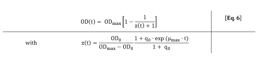
From Eq. 6, the parameters OD_max, q₀ and µ_max can be fitted to the OD600 data depicted in Fig. 3.

The fit of Eq. 6 to our OD600 data is shown in Fig. 7. As the OD600 profiles of rhamnose induction with 0.2% (w/v) and 0.5% (w/v) were similar, only the OD600 profile for 0.2% (w/v) was fitted to Eq. 6.

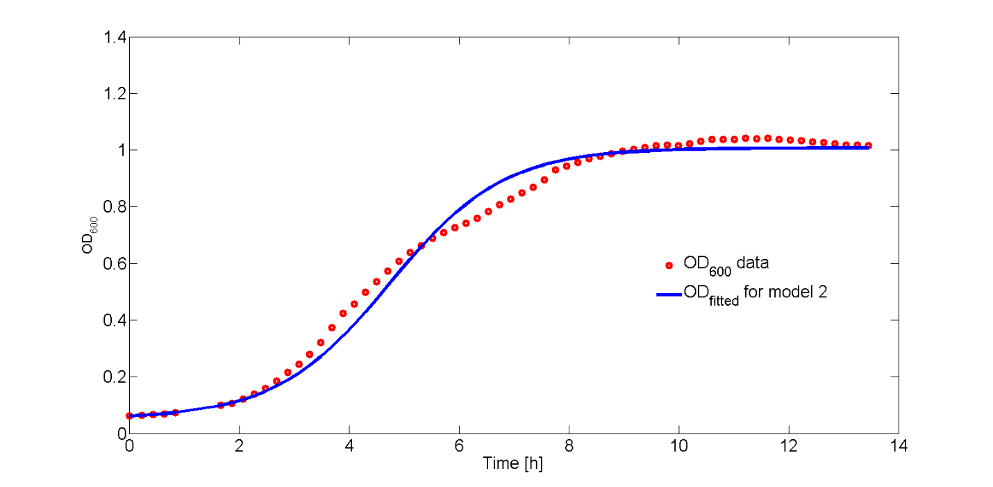
The fitted values for OD_max, q₀ and µ_max are:

From the fitted function of the OD600, an analytical expression for the growth rate can be derived. The growth rate is equal to:

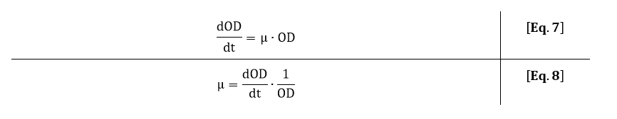
Filling in Eq. 5 in Eq. 8 gives the following expression for the growth rate:

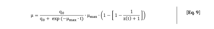
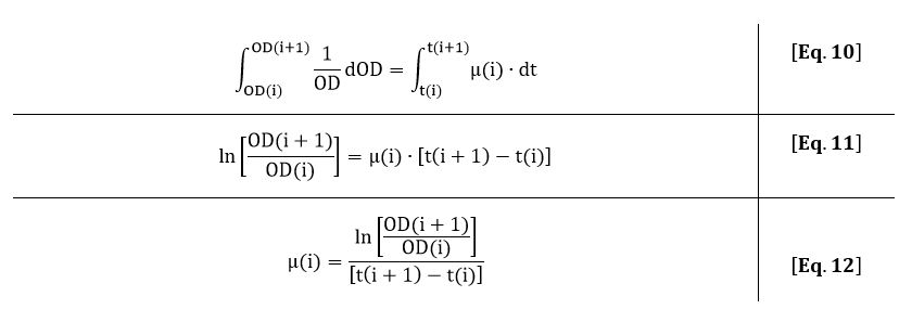
The growth rate can also be estimated from the OD600 by integrating Eq. 7:

In Fig. 8, the fitted growth rate as a function of time and the growth rate estimated from our data are both plotted.

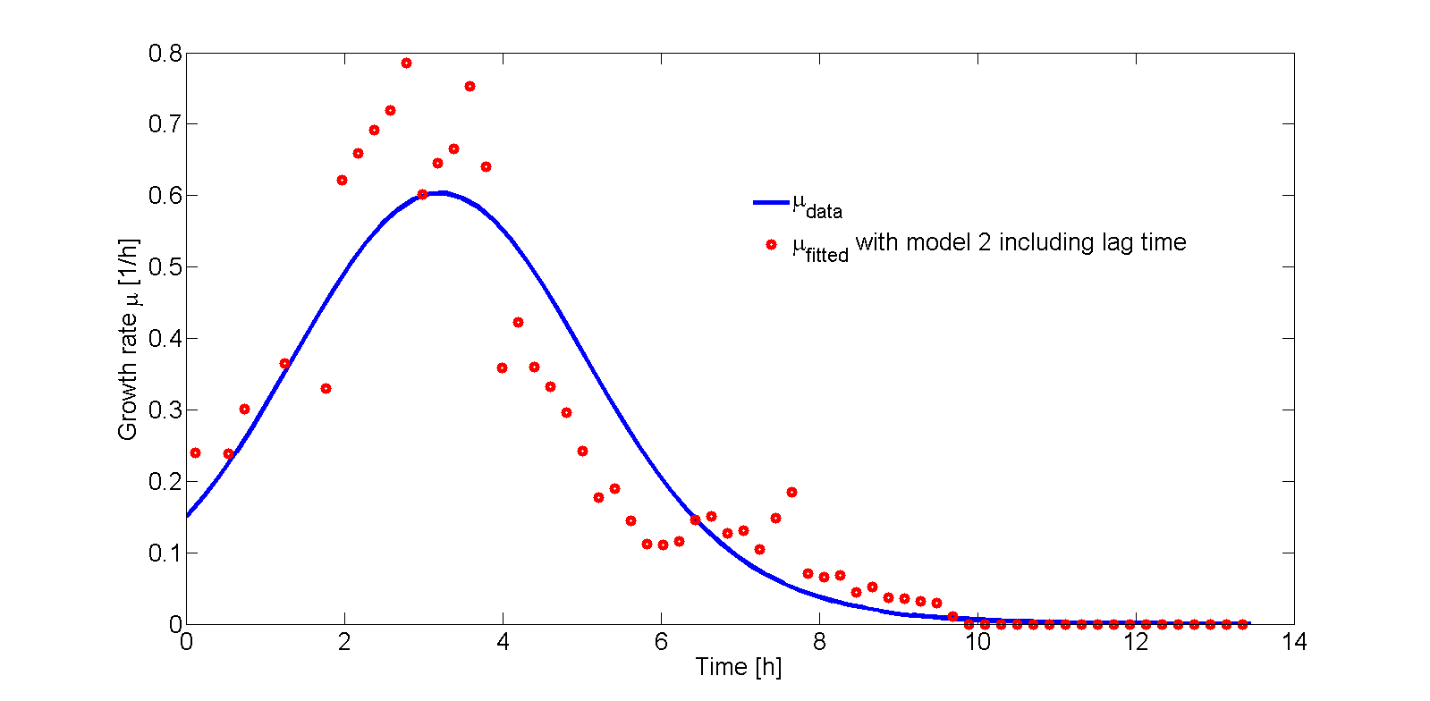
The difference between data and model can be explained by an approximation of the growth rate from the data or the error in the measurement of the plate reader. However, the growth rate function correctly describes the trend of the data.

As all the growth rate for our culture as a function of time is known, the GFPmut3 kinetic model can be applied to calculate the promoter activity for different levels of rhamnose induction. The following values were found:

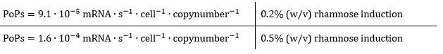
As can be derived from the PoPs values, the promoter is approximately 1.7 times more active when induced with 0.5% (w/v) rhamnose with respect to 0.2% (w/v) rhamnose. Now, the intracellular csgA concentration will be determined in order to relate these promoter activities to csgA production rates in molecules per second.

csgA intracellular concentration

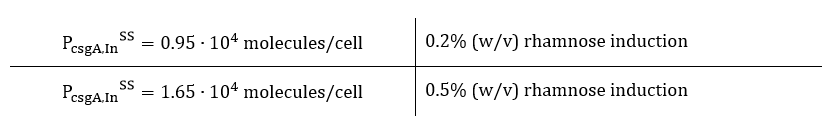
From the kinetic experimental data, the steady state concentration of GFP was 1.9∙104 molecules per cell for 0.2% (w/v) rhamnose induction and 3.3∙104 molecules per cell for 0.5% (w/v) rhamnose induction. As the csgA is transported to the extracellular space, the intracellular concentration of csgA (steady state) is not expected to be higher than the steady state concentration of GFP. Therefore, we estimate the steady state intracellular csgA concentration to be half the steady state concentration of GFP.

The intracellular steady state concentrations of csgA are thus:

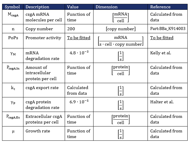
In order to calculate the csgA concentration in and outside the cell, a system of ordinary differential equations (ODE) needs to be defined. This model is similar to the GFP ODE system, except that the csgA is transported out of the cell. As the transporter protein (csgG) is not ATP dependent (van Gerven et. al), it can be assumed that the rate of csgA transport is dependent on the intracellular csgA concentration times a transport rate constant (kt). Furthermore, the translation rate of csgA is higher than the GFP translation rate. The translation rate of csgA is equal to:

The system of ODE’s describing csgA intracellular and extracellular concentration can be found in Table 2.

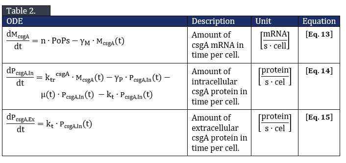
From Eq. 14, the steady state concentration of csgA can be calculated. As in steady state the accumulation of intracellular csgA is zero, the csgA transport rate can be written as:

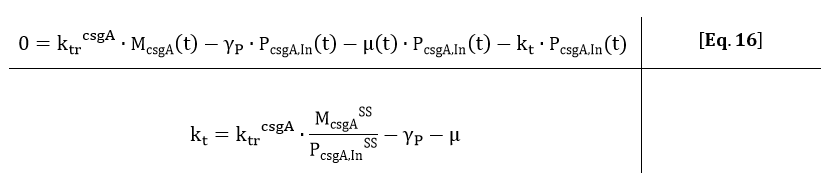
From the kinetic model, the PoPs was fitted to our data and can be used to calculate the steady state concentration of csgA mRNA:

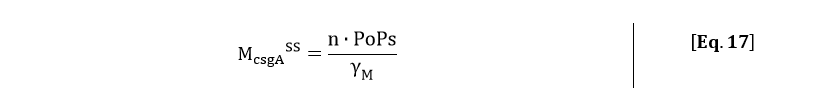
Filling in the steady state concentration of csgA mRNA gives:

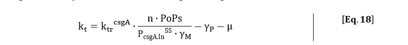
The degradation of csgA mRNA is assumed to be equal to the degradation of GFPmut3 mRNA. Furthermore, when the concentration of intracellular csgA has reached steady state, the growth rate of the culture will be close to zero as the culture will be in the stationary phase. Filling in the numbers in Eq. 18, gives a csgA transport rate constant of:

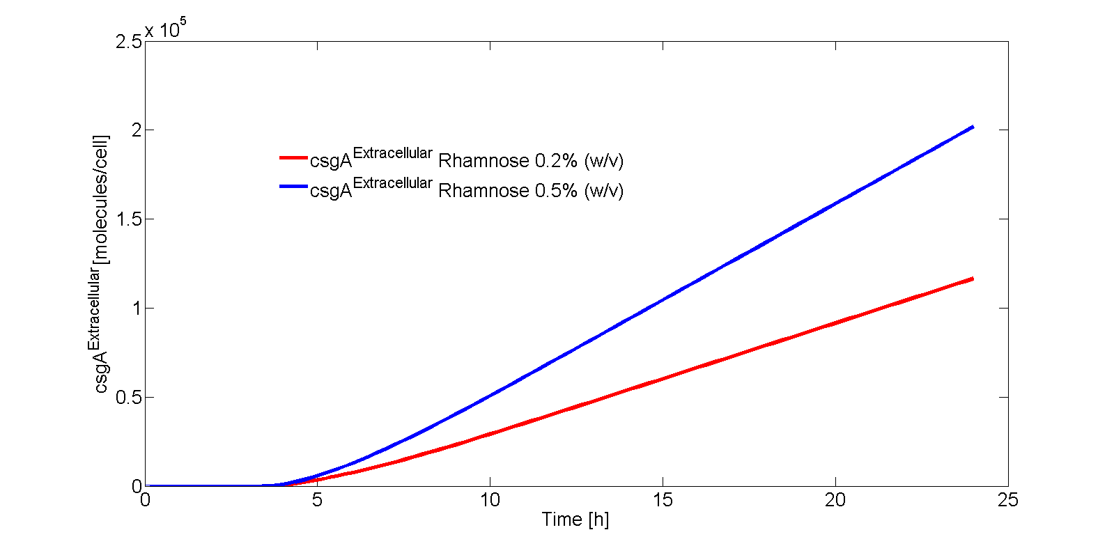
The extracellular csgA concentration can now be plotted as a function of time (Fig. 9).

If the intracellular concentration of csgA has reached steady state, the production of csgA is equal to:

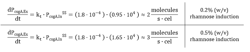
The extracellular concentration of csgA is thus equal to:

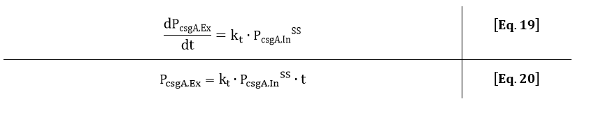
As can be seen from Eq. 20, if the intracellular concentration of csgA has reached steady state, the extracellular concentration of csgA will increase linearly in time (as can be also seen after 5 hours in Fig. 9).

As the production rate of csgA is in the order of 2-3 proteins per second, the csgA production will be limiting. This is because the number of csgB proteins in the outer membrane is more in the order of 100-1000 proteins csgB (Wang et. al). A higher induction level of rhamnose will produce more curlis, leading to a higher degree of curli intercellular connectivity and thus to a stronger biofilm. Therefore, with our inducible rhamnose promoter it is possible to control, to a certain degree, the biofilm strength of our printed samples.

Download a complete collection of all MATLAB files here

Back to Top

Curli Formation

In the formation of curlis, many factors play a role in determining the length and amount of curlis on one cell. These factors are for instance the rate of production of csgA, the amount of csgB proteins on the outer membrane and csgA diffusion. In the grid model, all three of these factors will be combined in order to determine what is limiting in curli formation. From our TEM photos, a parameter characterizing the behavior in curli growth will be estimated.

Results

In order to take both diffusion and curli formation into account, a mathematical grid model has been made. In this grid model, one grid element can either be a csgA molecule, csgB molecule, reactive curli end, part of a cell or part of a curli (Fig. 10).

In the model, csgA molecules are placed at a certain frequency. This frequency depends on the level of rhamnose induction, which was determined in section 1- kinetic modeling:

When the csgA molecule is placed on the grid, the csgA molecule can either:

I. Diffuse through the grid if it does not encounter a csgB or reactive curli end.

II. Bind to a csgB molecule, which starts the curli formation.

III. Bind to a reactive curli end, which increases the length of a curli.

Diffusion, I, is modelled as a random walk through the grid. The csgA molecule has 4 options: go one grid element up, down, left or right. In order to make the movement random, a random number between 0 and 1 is generated by MATLAB determining the direction of movement.

In Table 1 the outcome of csgA movement is indicated:

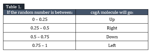
The csgA molecule will randomly diffuse through the grid until it encounters a csgB molecule (II) or reactive curli end (III).

For II, a reactive curli end is created. The curli chain thus becomes longer if more csgA diffuse to this reactive curli end (III).

The process of curli formation can thus be modelled, but without any modification to the model this could result in curli chains with very sharp turning angles (Fig. 11).

As this is not biologically possible, another parameter needs to be introduced controlling the growth of the curli chain. This parameter is called the “probability to turn” and can be varied from 0 to 1. If the probability parameter is set to 0, curli attachment is completely random. If the probability parameter is set to 1, the curlis grow only straight. Any other number between 0 and 1 is a combination between the two.

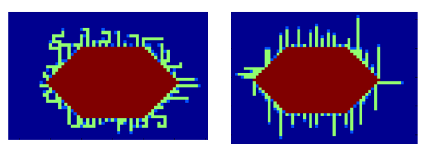
In Fig. 12 the result is shown for a probability factor of 0.6 and 1:

The probability to turn can be roughly estimated from our own TEM images, depicted in Fig. 13.

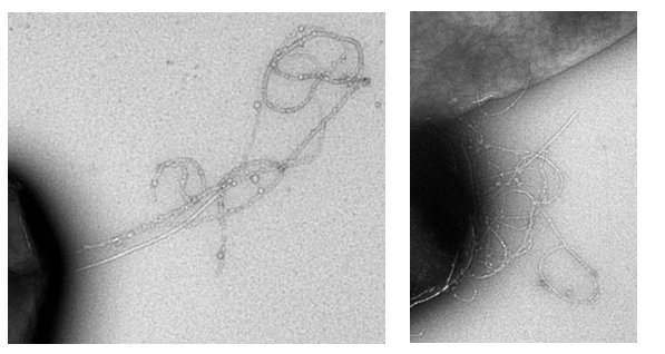
From Fig. 13 it can be seen that it is hard to determine one correct probability factor. For both TEM images it is however true that the curlis include large parts where growth is only in one direction. This would best fit a probability factor around 0.6.

Besides placing one cell on the grid, multiple cells can be placed on one grid. The number of simulations steps can be controlled by varying the parameter “R_max” in the MATLAB script. The script automatically makes a movie showing the curli growth. For an example simulation, click on the movie below!

The model further counts how many of the csgA molecules that are being produced, are actually part of the curlis.

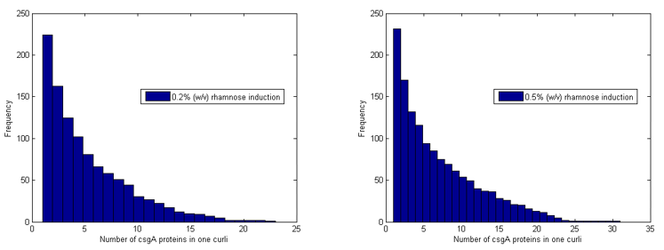
For both 0.2% (w/v) rhamnose induction and 0.5% (w/v) this is roughly the same. The absolute number of csgA attached to the curlis is however higher for a higher rhamnose induction level (Fig. 14).

As one grid element represent one csgA molecule, the importance of considering diffusion can be evaluated. One csgA molecule has a length of approximately 20 nm (Tian et al.). The diffusion constant of a protein is approximately 1∙10^-10 m²/s (bionumbers). This means that one characteristic step (τ) of a cgsA takes:

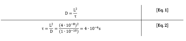
For 0.5% (w/v) rhamnose induction, 3 molecules of csgA per second are being produced. This means that for each production step of 3 molecules, a csgA molecule has moved 2.5∙10⁵ times on the grid. Due to this large difference in characteristic time, diffusion of csgA has almost no influence on the production time for one curli.

As the production for 0.2% (w/v) rhamnose induction is roughly 2 csgA molecules/cell and 3 csgA molecules/cell for 0.5% (w/v) rhamnose induction, 1.5 times more csgA molecules for 0.5% (w/v) rhamnose induction are able to take part in the curli formation for a certain period of time. However, we assume at first instance that this does not necessary has to lead to a stronger biofilm as the growth of curlis is fairly random. This is based on the probability factor of 0.6, which was found to be a good estimate in determining the curli growth direction. In the biofilm strength model, this initial assumption will be verified.

Download a complete collection of all MATLAB files here

Back to Top

Biofilm Strength

The kinetic model (section 1) and grid model (section 2) both predicted csgA production to be the limiting step. For current model, this information was used to be able to make a comparison between the biofilm strength of 0.2% (w/v) and 0.5% (w/v) rhamnose induction. As expected, the mean of curli connectivity was clearly higher for 0.5% (w/v) induction.

Model

The goal of this model, is to model the biofilm strength for different rhamnose induction levels. We define the biofilm strength as the degree of curli connectivity. In this model, we will count how many curlies will overlap for a certain amount of rhamnose induction. The more curlis overlapping, the higher the biofilm strength.

Our biofilm strength model is based on a worm-like chain model. With the use of Monte Carlo simulations, we generate random angels, which are Gaussian distributed. These random generated angels have a value that dependents on the persistence length. The persistence length is thus a parameter that will characterize the stiffness of our curli. The higher the persistence length, the greater the stiffness of our curli.

The mean (µ) of the random angles that are generated is 0, as locally the segments go straightforward. Furthermore, there is an equal chance that they bend to the right or to the left. The standard deviation (σ) of the angle distribution is:

As our biofilm strength model is in 3D, we have to generate two angles (ψ_u and ψ_v). With these angles, the csgA segment j is placed on the csgA segment j-1 in the axis of the last curli.

Before we can place the new segment on top, we have to calculate the direction of the last curli segment relative to the real x y and z axis. We start with the tangent unit vector |t| of the last segment j-1 . Out of this tangent vector, we can calculate the other two orthogonal unit vectors |u| and |v|.

Therefore, we first calculate the direction α (between zero and π) and azimuthal angle β (between zero and 2π) of the tangent vector as:

This angles we use to set up the tj, uj, vj axes of the new curli segment:

Now we can place the new segment with an angle relative to the created axes (tj, uj, vj). The next step is to calculate the tangent vector of the new segment. Therefore we have to decompose this vector into the three axes we defined ( tj, uj, vj )

The ct cu and cv are the coordinates we have to determine. Because we already know the angles of this new vector (the ψu and ψv angles we choose randomly), we know that:

Solving the three equations for the three unknown coefficients gives:

The last step is to save the new coordinates by adding the last segment to new direction times its length:

We let MATLAB grow the resulting curlis. At last, the overlap of only curlis from different cells is counted as connectivity. Namely, curlis from the same cell which are overlapping do not contribute to an increase in biofilm strength.

Results

In the kinetic modelling (section 1), the csgA production rates were determined:

Both the kinetic model and the grid model (section 2), predicted the csgA production to be the limiting step. Therefore, one of conclusion of the grid model was that 1.5 times more csgA proteins for 0.5% (w/v) rhamnose induction are able to take part in the curli formation for a certain period of time (with respect to 0.2% (w/v) induction level). In order to do so, in the MATLAB file “biofilm_strength_3D number” the number of segments was set to:

As the purpose of the model is to compare the biofilm strength for different induction levels relative to each other, the number of csgA segments were chosen arbitrary. However, the resulting curli length is in the order of micrometers, which is in the right order of magnitude (Pitkänen et al.). The biofilm strength was calculated for 4 cells, each cell having 5 curlis.

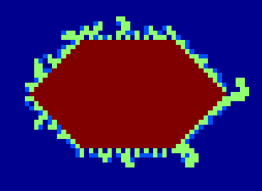
The persistence length can be estimated based on the TEM images in the same manner as in the grid model. A good estimate for the persistence length, based on these TEM images, is 400 nm. In Fig. 1, a simulation of the biofilm is shown for 0.2% (w/v) and 0.5% (w/v) rhamnose induction.

The model was executed 40 times; the average value of curlis connecting was 2.4 for the level of 0.2% (w/v) rhamnose induction and 5.8 for the level 0.5% (w/v) rhamnose induction. In 86% of the simulations, the connected amount of curlis was higher for 0.5% (w/v) induction. This means that there is a probability for the biofilm strength to be higher for 0.2% (w/v) rhamnose induction, although the contrary is more likely.

In conclusion, if the objective is to produce biofilms with different strengths, it is better to choose levels of rhamnose induction levels which are far apart. If the objective is to make a strong biofilm, a high level of rhamnose induction should be selected, as the csgA production is limiting.

Download a complete collection of all MATLAB files here

Time for Printing

In the section hardware, we characterized the velocity profile of our 3D printer. In order to make your figure of choice, the motors need to be pressed for a certain amount of time. In order to calculate these times, the MATLAB functions “Time_printer.m” and “Connect_points.m” have been written. These codes generate a text file which indicates how many seconds the motors have to be pressed to make a certain figure with our Biolinker.

Tutorial to printing time!

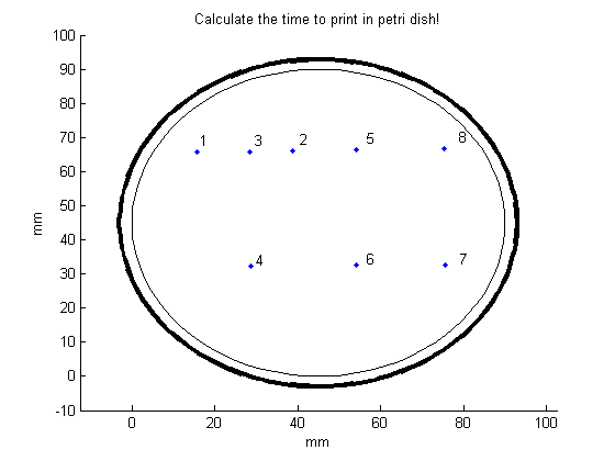
Let’s say, we want to print TU in the petri-dish with the Biolinker. At first, the number of points of this figure needs to be determined. To print TU you would need 8 points. The number of points can be set by changing the parameter “max_teller” in the file “Time_printer.m” (here: 8 points). When this parameter has been filled in, the file “Time_printer” can be run in MATLAB. After running, the file generates the following figure:

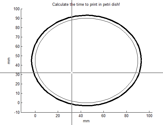
The middle of the cross indicates where the point will be placed after clicking. Click 8 times for making TU appear in the petri dish:

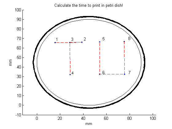
In order to make the desired figure more clear, open the function “Connect_points.m”. In this file, there are two input parameters.

The first input parameter is “line_to_be_removed”. Inside the squared brackets, list the points that should not be connected (here: points 4 and 5).

In the second input parameter, “time_to_press”, indicate with which gear you want to print. For the slow gear select “v_slow”, for the fast gear select “v_fast”. The “v” stands for the velocity of the needle, which has been measured for both gears. For the specifications of the measurements, go to the section “Hardware”.

To print TU in a petri dish, we will select the slow gear. The MATLAB file “Connect_ponts.m” can now be runned. The following figure will appear:

If the printed figure is satisfying enough, the printing times can be requested by clicking on the automatic generated test file “time_to_press”.

Opening the file “time_to_press.m” gives the following result:

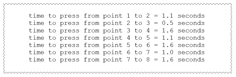
Now we know how much time we have to press our KNEX motors!

Download a complete collection of all MATLAB files here

References

“FACS-optimized mutants of the green fluorescent protein (GFP)”, Brendan P. Cormack, Raphael H. Valdivia and Stanley Falkow, Gene, 173 (1996) 33-38

“Automated Live Cell Imaging of Green Fluorescent Protein Degradation in Individual Fibroblasts”, Michael Halter, Alex Tona, Kiran Bhadriraju, Anne L. Plant, John T. Elliott, Cytometry Part A ,71A: 827-834, (2007)

“Optimization of an E. coli L-rhamnose-inducible expression vector: test of various genetic module combinations”, Angelika Wegerer, Tianqi Sun and Josef Altenbuchner, BMC Biotechnology 2008, 8:2

https://greenfluorescentblog.wordpress.com/tag/gfpmut3/, (2012)

“Measuring the activity of BioBrick promoters using an in vivo reference standard”, Jason R Kelly, Adam J Rubin, Joseph H Davis, Caroline M Ajo-Franklin, John Cumbers, Michael J Czar, Kim de Mora, Aaron L Glieberman, Dileep D Monie and Drew Endy, Journal of Biological Engineering 2009, 3:4

“Alternative Approach To Modeling Bacterial Lag Time, Using Logistic Regression as a Function of Time, Temperature, pH, and Sodium Chloride Concentration”, Shige Koseki and Junko Nonaka, FEMS Yeast Res 14 (2014) 586–600

“Gatekeeper residues in the major curlin subunit modulate bacterial amyloid fiber biogenesis”, Xuan Wang, Yizhou Zhou, Juan-Jie Ren, Neal D. Hammer, and Matthew R. Chapman, PNAS, (2010), vol. 107., no.1, 163-168

http://parts.igem.org/Part:BBa_K914003

Secretion and functional display of fusion proteins through the curli biogenesis pathway, Van Gerven N, Goyal P, Vandenbussche G, De Kerpel M, Jonckheere W, De Greve H, Remaut H, Molecular Microbiology (2014) 91(5), 1022–1035

“Nanofibrillar cellulose – in vitro study of cytotoxic and genotoxic properties", Pitkänen, M. et al, VTT Technical Research Center of Finland.

"An open-source software tool to determine the mechanical properties of worm-like chains",Lamour G, Kirkegaard JB, Li H, Knowles TP, Gsponer J. Easyworm, Source Code for Biology and Medicine, (2014)

“Structure of a Functional Amyloid Protein Subunit Computed Using Sequence Variation”, Pengfei Tian, Wouter Boomsma, Yong Wang, Daniel E. Otzen, Mogens H. Jensen and Kresten Lindorff-Larsen, University of Copenhagen, 2014.

http://kirschner.med.harvard.edu/files/bionumbers/fundamentalBioNumbersHandout.pdf

Team:TU Delft/Modeling

Modeling

Overview

Kinetic Modeling

csgA production rate

csgA intracellular concentration

Curli Formation

Results

Biofilm Strength

Model

Results

Time for Printing

Tutorial to printing time!

Now we know how much time we have to press our KNEX motors!

References