Team:Tuebingen/Modeling

The objective of our project was to build a population-encoding galactose sensor with the ability to measure and store the concentration level at one specific time-point. The temporal selectivity of the sensor was achieved by light-induced conformational changes of Dronpa, which is a monomeric fluorescence protein. Its fluorescence is activated by violet light (400nm) and deactivated by cyan light (500nm). Dronpa tetramerizes in the fluorescing 'ON'-state. [Zhou2012]
We utilized Dronpa’s behavior to introduce light-dependent regulation to Cre monomers, which tetramerize to a recombinase complex. In our chassis, the Cre recombinase deletes RFP, which prevents the transcription of a luciferase reporter. The mechanism of our sensor is the galactose dependent expression of Dronpa (in the ON state), which after the exposure to 500nm light no longer inhibits the recombinase. Consequently, a Cre-Lox recombination deletes RFP, which activates the reporter.
A recombinase event could be considered a stochastic process, that depends on the Cre concentration and on the time span in which it was active. Because the concentration of Dronpa and of the linked Cre is determined by the galactose concentration, the change in luciferase activity in a population is a measure of the galactose concentration at the time point of 500nm light exposure.
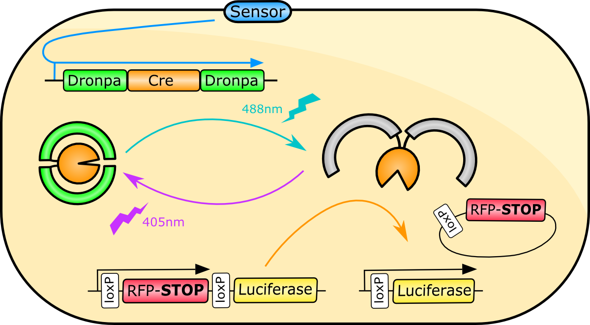
Figure 1: Overview of the chassis

Figure 1: The dynamic species and their interactions in the model
Our model is based on the constructs pGAL - NLS - Dronpa - Cre-Dronpa and PADH - RFP - Luciferase. The variable parts of the model are depicted in the upper diagram. We assume that the PADH mediated expression and the overall Dronpa concentration are constant.
Table 1: Abbreviations for the genetic elements:
| Genetic Element | Description |
|---|---|
| pGAL | [Galactose] dependent promoter |
| Dronpa | Dronpa monomer |
| NLS | Signal for nucleus import |
| Cre | Cre monomer |
| PADH | Promotor with constant expression |
| RFP | Inhibits reporter expression |
| Luciferase | Reporter |
We described the dynamics of the system with the following equations.
\(\begin{eqnarray} \frac {\partial \left[ \textrm{Dronpa}_\textrm{On}\textrm{-Cre} \right]} {\partial t} &=& \left(\textrm{Off}\rightarrow\textrm{On}\right) - \left(\textrm{On}\rightarrow\textrm{Off}\right)\\ & & \\ &=& \alpha \cdot \left[ \textrm{Dronpa}_\textrm{Off}\textrm{-Cre} \right] \cdot [400nm] \\ & & - \beta \cdot \left[ \textrm{Dronpa}_\textrm{On}\textrm{-Cre} \right] \cdot [500nm] \end{eqnarray}\)
\(\begin{eqnarray} \frac {\partial \left[ \textrm{Dronpa}_\textrm{Off}\textrm{-Cre} \right]} {\partial t} &=& \left(\textrm{On}\rightarrow\textrm{Off}\right) - \left(\textrm{Off}\rightarrow\textrm{On}\right) & & \\ &=& \beta \cdot \left[ \textrm{Dronpa}_\textrm{On}\textrm{-Cre} \right] \cdot [500nm] \\ & & - \alpha \cdot \left[ \textrm{Dronpa}_\textrm{Off}\textrm{-Cre} \right] \cdot [400nm] \end{eqnarray}\)
| Parameter/Species | Unit | Function |
|---|---|---|
| \([500nm]\), \([400nm]\) | \(\frac{photons}{sec}\) | Light intensities |
| \(\alpha\) | \(\frac{1}{photons}\) | Scaling factor |
| \(\beta\) | \(\frac{1}{photons}\) | Scaling factor |
Let \(A = \int\ [\textrm{Dronpa}_\textrm{Off}\textrm{-Cre}]_t\ dt\) be the area under \(\textrm{Dronpa}_\textrm{Off}\) concentration curve.
The area \(A\) describes how much and how long Cre was active. As such it could be used as a measure for the likelihood of a recombinase event occurring in a single cell. We suspected a sigmoidal relationship between the integral and the probability of a recombinase event occurring in a single cell.
According to the Binomial distribution, if a tube contained \(N\) cells that had no reporter activity, the expected number of recombinase events after light exposure is \(N \cdot f(A)\). As we assumed constant PADH expression, each of these cells will have about the same luciferase concentration. Therefore we can predict the change in luciferase luminescence \(L\) do be proportional to \(N \cdot f(A)\). (The yeast is on a plate, and therefore has a constant distance to the measurement device)
If \(k\) is the proportionality coefficient in \(L = k \cdot N \cdot f(A)\) for an observed \(L\), then it is \(A = f^{-1} \left(\frac{L}{k\cdot N}\right)\). From \(A\), we were able to deduce \([\textrm{Dronpa}_\textrm{On}]\) at the time point of light exposure, which allows the computation of the galactose concentration as we assumed that a Hill function describes the Dronpa expression.
In our chassis, the sensor platform is the promoter pGAL, which originates from the gal operon. As such pGAL has the function of a switch, which according to Kim et al. [Kim 2012], could be described with a Hill function.
The hill function is:\(\begin{eqnarray} \frac {\partial \left[ \textrm{Dronpa}_\textrm{On}\textrm{-Cre} \right]_\textrm{production rate}} {\partial t} &=& V : \left(\frac {K^n} {[GAL]^n} + 1 \right)\\ \end{eqnarray}\)
| Parameter/Species | Unit | Function |
|---|---|---|
| \(V\) | \(\frac {M}{sec}\) | Max. production-rate of Dronpa |
| \(K\) | \(M\) | Steepness of Hill function |
| \(n\) | none | Hill coefficient |
Since the model will only cover a short timespan, in which the Dronpa concentration is constant, we were interested in the steady-state concentrations. A steady state implies the presence of a decay of the molecules. An exponential decay with half-life time \(\tau\) is described by the following equation.
\(\begin{eqnarray} \frac {\partial \left[ \textrm{Dronpa}_\textrm{On}\textrm{-Cre} \right]_\textrm{decay rate}} {\partial t} &=& -\frac{\ln(2)}{\tau} \left[ \textrm{Dronpa}_\textrm{On}\textrm{-Cre} \right] \\ \end{eqnarray}\)
In a steady state, the production rate equals the decay.
\(\begin{eqnarray} V : \left(\frac {K^n} {[GAL]^n} + 1 \right) &=& \frac{\ln(2)}{\tau} \left[ \textrm{Dronpa}_\textrm{On}\textrm{-Cre} \right]_\textrm{s.s} \\ \Rightarrow \left[ \textrm{Dronpa}_\textrm{On}\textrm{-Cre} \right]_\textrm{s.s} &=& \underbrace{ \frac {V \cdot \tau} {\ln(2)} }_{V'} : \left(\frac {K^n} {[GAL]^n} + 1 \right) \end{eqnarray}\)
For a given \(V'\), \(\tau\) and \(V\) are inversely proportional. Therefore, we did not need to explicitly determine these parameters, because their product is sufficient to determine the steady state concentration.
According to Hippler et al, 2003, photochemical reactions can be modeled as a zeroth order kinetics with the following rates.
\(\begin{eqnarray} v_{\textrm{Off}\rightarrow\textrm{On}} &=& \alpha \cdot \left[ \textrm{Dronpa}_\textrm{Off}\textrm{-Cre} \right] \cdot [400nm] \\ \end{eqnarray}\)
\(\begin{eqnarray} v_{\textrm{On}\rightarrow\textrm{Off}} &=& \beta \cdot \left[ \textrm{Dronpa}_\textrm{On}\textrm{-Cre} \right] \cdot [500nm] \\ \end{eqnarray}\)
These kinetics show an exponential profile for the concentration over time plot. Therefore, the amount Dronpa\(_\textrm{On}\) remaining after a 500nm light impulse of \(t_1\) duration is:
\(\begin{eqnarray} \left[ \textrm{Dronpa}_\textrm{On}\textrm{-Cre} \right]_{t_1} &=& \int_0^t - \beta \cdot [500nm] \cdot \left[ \textrm{Dronpa}_\textrm{On}\textrm{-Cre} \right]_{t'} dt'\\ &=& \left[ \textrm{Dronpa}_\textrm{On}\textrm{-Cre} \right]_{s.s.} \cdot \exp\{-\beta\cdot [500nm] \cdot t_1\} \end{eqnarray}\)

Figure 1: Schematic profile of the Dronpa-Off curve.
Under the Assumption that the \([\textrm{Dronpa}_\textrm{Off}\textrm{-Cre}]\) after the last light impulse is negligibly small, the area under the curve is easily derivable from the exponential profiles.
\begin{eqnarray} A &=& \enclose{circle}{1} + \enclose{circle}{2} + \enclose{circle}{3}\\ &=& \int_0^{t_1} \left[ \textrm{Dronpa}_\textrm{Off}\textrm{-Cre} \right]_{t'} dt' \\ &&+ t_2 \cdot \left[ \textrm{Dronpa}_\textrm{Off}\textrm{-Cre} \right]_{t_1} \\ &&+ \left[ \textrm{Dronpa}_\textrm{Off}\textrm{-Cre} \right]_{t_1} \int_0^{t_3} \exp\{-\alpha[400nm]t'\} dt' \\ &=& \int_0^{t_1} \left[ \textrm{Dronpa}_\textrm{On}\textrm{-Cre} \right]_{s.s.} - \left[ \textrm{Dronpa}_\textrm{On}\textrm{-Cre} \right]_{t'} dt' \\ &&+ t_2 \cdot \left( \left[ \textrm{Dronpa}_\textrm{On}\textrm{-Cre} \right]_{s.s.} - \left[ \textrm{Dronpa}_\textrm{On}\textrm{-Cre} \right]_{t_1} \right) \\ &&+ \left( \left[ \textrm{Dronpa}_\textrm{On}\textrm{-Cre} \right]_{s.s.} - \left[ \textrm{Dronpa}_\textrm{On}\textrm{-Cre} \right]_{t_1} \right) \cdot \int_0^{t_3} \exp\{-\alpha[400nm]t'\} dt' \\ &=& \left[ \left[ \textrm{Dronpa}_\textrm{On}\textrm{-Cre} \right]_{s.s.} \cdot \left( t' - \frac{\exp\{-\beta[500nm]t'}{-\beta[500nm]}\} \right) \right]^{t_1}_0\\ &&+ t_2 \cdot \left[ \textrm{Dronpa}_\textrm{On}\textrm{-Cre} \right]_{s.s.} \cdot \left( 1 - \exp\{-\beta[500nm]t_1\} \right)\\ &&+ \left[ \textrm{Dronpa}_\textrm{On}\textrm{-Cre} \right]_{s.s.} \cdot \left( 1 - \exp\{-\beta[500nm]t_1\} \right) \cdot \left[ \frac{\exp\{-\alpha[400nm]t'\}}{-\alpha[400nm]} \right]^{t_3}_0\\ &=& \left[ \textrm{Dronpa}_\textrm{On}\textrm{-Cre} \right]_{s.s.} \cdot \big( t_1 - \frac 1 {\beta[500nm]} + \exp\{-\beta[500nm]t_1\} \cdot \\&& \left( \frac 1 {\beta[500nm]} + t_2 - \frac {\exp\{-\alpha[400nm]t_3\}}{\alpha[400nm]} + \frac 1 {\alpha[400nm]} \right) \big)\\ &\propto& \left[ \textrm{Dronpa}_\textrm{On}\textrm{-Cre} \right]_{s.s.} \end{eqnarray} $
The Chemwiki suggests that the concentration of fluorescent proteins is proportional to the fluorescence signal, if only a fraction of the excitation energy is absorbed, which is the case for our project. Consequently, the last equation shows that this coefficient will only scale the total area, and therefore can be omitted.
Side-note concerning the ‘concentration of light’: light is specified as photons per second. For a laser of energy \(W\) the Max-Planck law states \(W=nE = nhv \Rightarrow n = \frac W {hv}\) for the wave frequency \(v\).
In a time series experiment, we found the reaction time for protein expression of pGal-Luciferase to take \(7-8h\). Therefore, we conducted experiments for determining the the steady-state expression levels for different galactose concentrations. Unfortunately, we could neither use the observations to fit the parameters of the pGAL promoter nor could we--due to technical limitations--build a fully functional chassis. (see figures below)
However, an experiment yielded steady-state solutions for pSUC, a promoter which is repressed by glucose. We were able to compute a semi-reasonable fitting of a hill function (\(R^2=0.61\)); we suggest that this could be seen as a proof of concept for the suggested equation of the sensor platform.
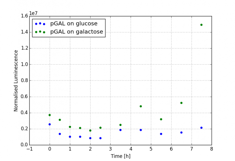
Figure 1: Shown is the progression of expression for a GAL--Luciferase construct over time under various medium conditions.
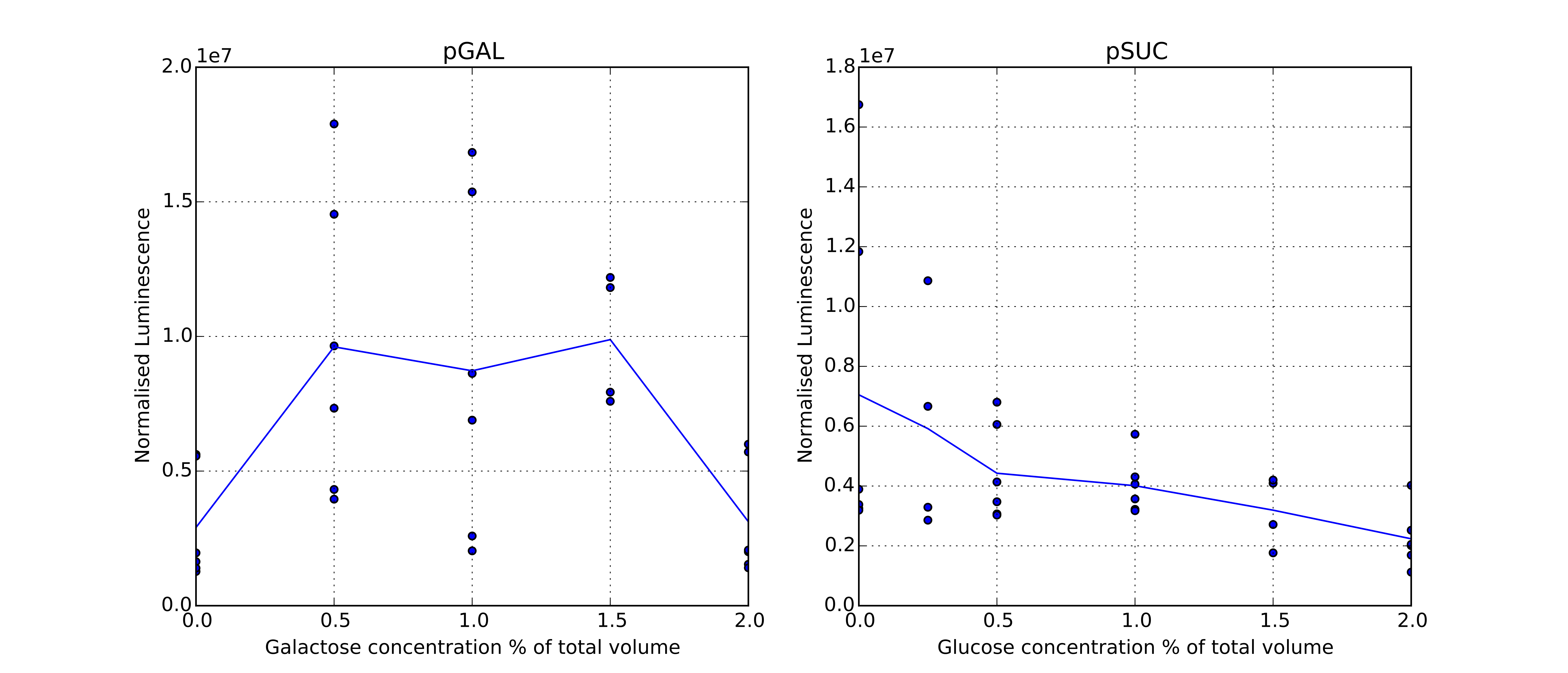
Figure 2: The plots show the normalised luciferase expression after an overnight cultivation for various substrate concentration levels. The lines connect the arithmetic means per level.
The values were sample-wise (per plates) z-normalised. The curve fitting was performed with matlab’s cftool.
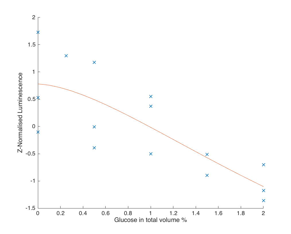
Figure 3: Shown is a fitted hill function that was based on the z-normalised luminescence values of pSUC.
The parameters were:
\(\begin{eqnarray} f(x) = \frac {v} { \left(\frac k x\right)^n + 1} + c \end{eqnarray}\)
| Parameter | Value |
|---|---|
| v | 5.565 |
| k | 3.028 |
| n | -1.615 |
| c | -4.784 |
Concerning the modeling of Dronpa’s On/Off-transition: We were only able to utilise a laser-scanning microscope to turn Dronpa off and back on again. We utilised Fiji to fit circles around cells and to quantify the background and foreground signal level (similar to the pre-processing of a spotted micro-array). After performing intra-measurement normalisation with global scaling (z-transformation), no pattern was visible in the background corrected signal (by subtraction) over time. Therefore, we were unable to verify the assumption of 0-th kinetics for the photochemical reactions.

Figure 4: Boxplot comparison of the continuous microscopy measurements.Left are the raw background corrected values, and right the globally scaled values.