Difference between revisions of "Team:Oxford/Modeling"
| Line 12: | Line 12: | ||
<h2>Introduction</h2> | <h2>Introduction</h2> | ||
<p> | <p> | ||
| − | Mathematical | + | Mathematical <a class="definition" title="model" data-content="A simplified or idealised description of a system or process, usually mathematical, that can be used to predict how it will behave.">model</a>ling plays a crucial role in Synthetic Biology by acting as a link between the conception and the physical realisation of a biological circuit. Our modelling team has focused on building a better picture of the project to evaluate the effectiveness of initial designs, as well as to provide insight into how the system can (or must) be improved. To do this we have split our modelling efforts into three main sections: <em>Characterising our Cells</em>, <em>Interaction with the Environment</em>, and <em>Interaction with the Biofilm</em>. By combining the information gathered in each of these section we hope to ultimately answer the question: Is our system feasible? If not, where should the design be altered? |
</p> | </p> | ||
<p> | <p> | ||
| Line 27: | Line 27: | ||
<h3>Arabinose Induced</h3> | <h3>Arabinose Induced</h3> | ||
<p> | <p> | ||
| − | We have decided to use an arabinose induced promoter for the expression of a number of our | + | We have decided to use an arabinose induced <a class="definition" title="promoter" data-content="The section of DNA that the RNA polymerase enzyme binds to before it starts making the RNA strand - it is needed to start transcription, so it sits in the DNA before a gene. Regulates whether a gene is "on" or "off" and to what extent. They can be made to be sensitive to certain conditions so that if a bacterium senses a change in environment it can up or down regulate the expression of a certain gene (so there will be more or less of the protein encoded by that gene, produced in the cell).">promoter</a> for the expression of a number of our <a class="definition" title="protein" data-content="An essential part of all living organisms. They are long and fold up into complicated structures and are made up of amino acids.">protein</a>s. This promoter can be modelled as the following chemical system: |
</p> | </p> | ||
| Line 33: | Line 33: | ||
\[mRNA\overset{\gamma_{1}}{\rightarrow}\phi\quad P\overset{\gamma_{2}}{\rightarrow}\phi\] | \[mRNA\overset{\gamma_{1}}{\rightarrow}\phi\quad P\overset{\gamma_{2}}{\rightarrow}\phi\] | ||
<p> | <p> | ||
| − | You can find out more information about how this promoter works here. For this system we will assume that AraC is always in large concentration and that its binding to arabinose happens on a faster time scale to transcription. Therefore, we do not need to consider the individual concentrations of arabinose and AraC, instead we just need to include the concentration of the complex [Arab:AraC]. The rate \(K\) is not just a simple constant and is given as the hill function in the equations below. | + | You can find out more information about how this promoter works here. For this system we will assume that AraC is always in large concentration and that its binding to arabinose happens on a faster time scale to <a class="definition" title="transcription" data-content="Process of synthesising RNA or DNA from an existing strand of DNA. The process of copying target DNA sequences onto RNA.">transcription</a>. Therefore, we do not need to consider the individual concentrations of arabinose and AraC, instead we just need to include the concentration of the complex [Arab:AraC]. The rate \(K\) is not just a simple constant and is given as the hill function in the equations below. |
</p> | </p> | ||
<p> | <p> | ||
| Line 220: | Line 220: | ||
</div> | </div> | ||
<p> | <p> | ||
| − | To calculate if our project will work in real life, we can model the number of cells required to reach a sufficient enzyme secretion rate to stop a biofilm from forming. To do this, we need to measure the rate of secretion of enzymes from our cells. | + | To calculate if our project will work in real life, we can model the number of cells required to reach a sufficient <a class="definition" title="enzyme" data-content="A molecule which speeds up a chemical reaction - a biological catalyst. The reaction does not involve these molecules.">enzyme</a> secretion rate to stop a <a class="definition" title="biofilm" data-content="A community of bacteria (or other microorganisms) adhering to a surface and each other, held together by secreted slime-like polymers that create a more favorable environment for the bacteria and protect them from environmental stresses and attack from a host’s immune system (in the case of pathogenic bacteria).">biofilm</a> from forming. To do this, we need to measure the rate of secretion of enzymes from our cells. |
</p> | </p> | ||
<p> | <p> | ||
| − | This can be difficult to do when the protein itself is mixed in with the fluid our cells grow in. GFP is much easier to measure in the lab, so we induced its expression and measured the fluorescence. From this we can find the parameters given in our first table, and then apply the model to a longer - or shorter - gene and predict expression. | + | This can be difficult to do when the protein itself is mixed in with the fluid our cells grow in. GFP is much easier to measure in the lab, so we induced its expression and measured the fluorescence. From this we can find the parameters given in our first table, and then apply the model to a longer - or shorter - <a class="definition" title="gene" data-content="A section of DNA which codes for a protein.">gene</a> and predict expression. |
</p> | </p> | ||
<p> | <p> | ||
| Line 232: | Line 232: | ||
<img src="https://static.igem.org/mediawiki/2015/d/de/OxiGEM_Gene_Fitter.png" alt="Fitting our gene expression data to the theoretical model" /> | <img src="https://static.igem.org/mediawiki/2015/d/de/OxiGEM_Gene_Fitter.png" alt="Fitting our gene expression data to the theoretical model" /> | ||
<p> | <p> | ||
| − | Graph depicting results of GFP concentration as a function of time, matched to our deterministic model. Errors are given to one standard deviation and an arbitrary scaling factor is employed. | + | Graph depicting results of GFP concentration as a function of time, matched to our <a class="definition" title="deterministic model" data-content="A deterministic model predicts a single outcome from a given set of circumstances.">deterministic model</a>. Errors are given to one standard deviation and an arbitrary scaling factor is employed. |
</p> | </p> | ||
</div> | </div> | ||
| Line 245: | Line 245: | ||
<h2>Delivery</h2> | <h2>Delivery</h2> | ||
<p> | <p> | ||
| − | With the information about the rates of production and concentrations of our products we can look at how the products behave once they leave the cell. This involves modelling the diffusion of the products in different topologies, each associated with a potential physical design of the catheter. With this information we can provide a better estimate of the time scale that our project is working on and assess any need for optimisation. | + | With the information about the rates of production and concentrations of our products we can look at how the products behave once they leave the cell. This involves modelling the diffusion of the products in different topologies, each associated with a potential physical design of the <a class="definition" title="catheter" data-content="A small, flexible tube inserted into the body to remove fluid. Urinary tract infections are a common side effect of using these.">catheter</a>. With this information we can provide a better estimate of the time scale that our project is working on and assess any need for optimisation. |
</p> | </p> | ||
<div id="delivery-dispersin"> | <div id="delivery-dispersin"> | ||
| Line 264: | Line 264: | ||
</p> | </p> | ||
<p> | <p> | ||
| − | To determine the convection mass transfer coefficient of Dispersin B from our gel spheres we looked at the diffusion data obtained from <a href="https://2015.igem.org/Team:Oxford/Beads#03-09-2015">this experiment</a> involving the diffusion of crystal violet from our beads. By analysing the system we can produce a theoretical form for the concentration of crystal violet in the bulk water as a function of time: | + | To determine the convection mass transfer coefficient of Dispersin B from our gel spheres we looked at the diffusion data obtained from <a href="https://2015.igem.org/Team:Oxford/Beads#03-09-2015">this experiment</a> involving the diffusion of <a class="definition" title="crystal violet" data-content="A staining chemical used to mark cell structures and make them more visible under light microscopy. It is also the chemical used in Gram’s staining method for classifying bacteria into those that are Gram positive (the cell walls are stained) and Gram negative (the cell walls are not stained).">crystal violet</a> from our beads. By analysing the system we can produce a theoretical form for the concentration of crystal violet in the bulk water as a function of time: |
</p> | </p> | ||
Revision as of 16:12, 17 September 2015
Modelling
Introduction
Mathematical modelling plays a crucial role in Synthetic Biology by acting as a link between the conception and the physical realisation of a biological circuit. Our modelling team has focused on building a better picture of the project to evaluate the effectiveness of initial designs, as well as to provide insight into how the system can (or must) be improved. To do this we have split our modelling efforts into three main sections: Characterising our Cells, Interaction with the Environment, and Interaction with the Biofilm. By combining the information gathered in each of these section we hope to ultimately answer the question: Is our system feasible? If not, where should the design be altered?
To help readers of all kinds and specialisations understand this page we have produced guides for all the modelling techniques used in this section which are available on the Modelling Tutorial page and will be linked to when relevant on this page.
Characterising Our Cells
In this section we look at our cells in isolation in order to assess their functionality and answer important questions such as “How long does it take to produce a certain concentration of product?”, and “What are the main limiting rates/concentrations?”. The first will help us assess the feasibility of our project, ie are our cells too slow? The second will aid us in further optimising our design.
Arabinose Induced
We have decided to use an arabinose induced promoter for the expression of a number of our proteins. This promoter can be modelled as the following chemical system:
\[[Arab:AraC]\overset{K}{\rightarrow}mRNA\overset{\alpha}{\rightarrow}P\] \[mRNA\overset{\gamma_{1}}{\rightarrow}\phi\quad P\overset{\gamma_{2}}{\rightarrow}\phi\]You can find out more information about how this promoter works here. For this system we will assume that AraC is always in large concentration and that its binding to arabinose happens on a faster time scale to transcription. Therefore, we do not need to consider the individual concentrations of arabinose and AraC, instead we just need to include the concentration of the complex [Arab:AraC]. The rate \(K\) is not just a simple constant and is given as the hill function in the equations below.
Using this approximation, we arrive at the equations:
\[\dfrac{d[mRNA]}{dt}=K_{max}\dfrac{[Arab:AraC]^{n}}{K_{half}^{n}+[Arab:AraC]^{n}}-\gamma_{1}[mRNA]\] \[\dfrac{d\left[P\right]}{dt}=\alpha\left[mRNA\right]-\gamma_{2}\left[P\right]\]Where we define the symbols as:
| Symbol | Definition | Initial Value/Literature Value | Fitted |
|---|---|---|---|
| \([Arab:AraC]\) | The concentration of associated Arabinose and AraC | \(0\) | - |
| \([mRNA]\) | The concentration of mRNA | \(0\) | - |
| \([P]\) | The concentration of our product | \(0\) | - |
| \(\alpha\) | Translation rate | \(15ntd\: s^{-1}\)/length of sequence [6] | ? |
| \(\gamma_{1}\) | Degradation rate of mRNA | \(5.13\times10^{-4}s^{-1}\) [5] | ? |
| \(\gamma_{2}\) | Degradation rate of product | \(5.13\times10^{-4}s^{-1}\) [5] | ? |
| \(K_{max}\) | Maximal transcription rate | \(50ntd\: s^{-1}\)/length of sequence [6] | ? |
| \(K_{half}\) | Half-maximal transcription rate | \(160\mu M\) [8] | ? |
| \(n\) | Hill coefficient | \(2.65\) [3] | ? |
This table contains literature values for the parameters, found from a number of sources. Later we will fit the parameters to the experimental data found by the wet lab team. For now though we can plot the expression graphs using the literature values. This will provide an estimate to the time scales involved.
There are mutliple products being expressed using this inducer-promoter pair, each of different sequence lenghts. Here is a table showing the relevant proteins and sequence lengths:
| Product | Sequence Length (/bp) |
|---|---|
| pBAD HisB DNase DsbA | 621 |
| pBAD HisB DspB YebF | |
| pBAD HisB DspB | |
| pBAD HisB MccS | 414 |
| pBAD HisB DspB Fla | |
| pBAD HisB Art-175 DsbA | 987 |
| pBAD HisB Art-175 YebF | 1284 |
| pBAD HisB Art-E | 632 |
| pBAD HisB Art-175 Fla | 1095 |
| pBAD HisB Art-175 | 936 |
| pBAD HisB DNase | 570 |
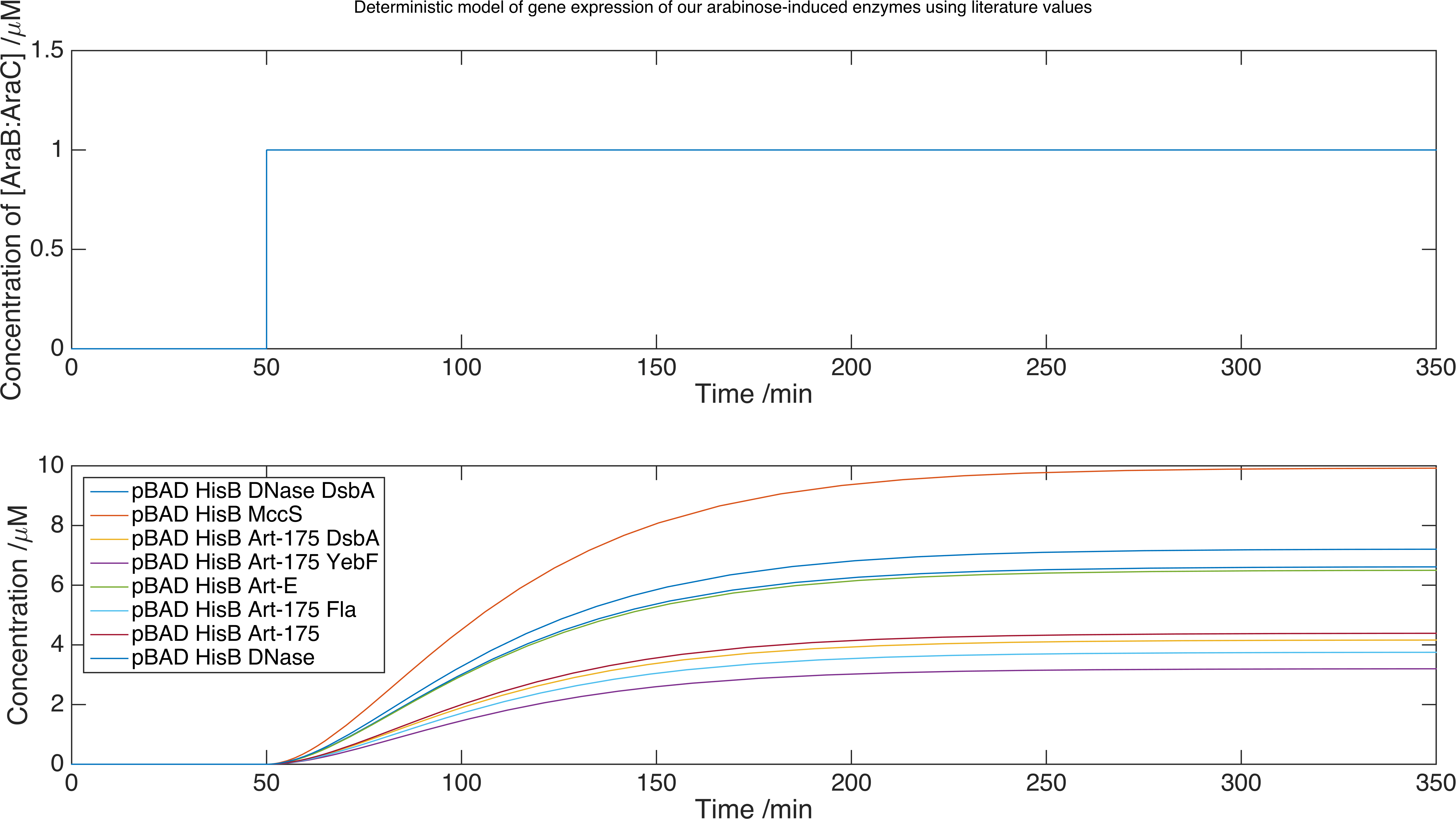
We now can run our model of the system by solving the set of equations using the MATLAB equation solver ode15s. Below is a plot of the concentration of product against time for each protein expressed with this inducer-promoter pair where the expression is induced by a step function:
To calculate if our project will work in real life, we can model the number of cells required to reach a sufficient enzyme secretion rate to stop a biofilm from forming. To do this, we need to measure the rate of secretion of enzymes from our cells.
This can be difficult to do when the protein itself is mixed in with the fluid our cells grow in. GFP is much easier to measure in the lab, so we induced its expression and measured the fluorescence. From this we can find the parameters given in our first table, and then apply the model to a longer - or shorter - gene and predict expression.
Using the graph below, we can fit our expression data to the model presented in the tutorial, where we have included an arbitrary scaling factor (instead of a calibration curve) to match GFP fluorescence to molecule concentrations.
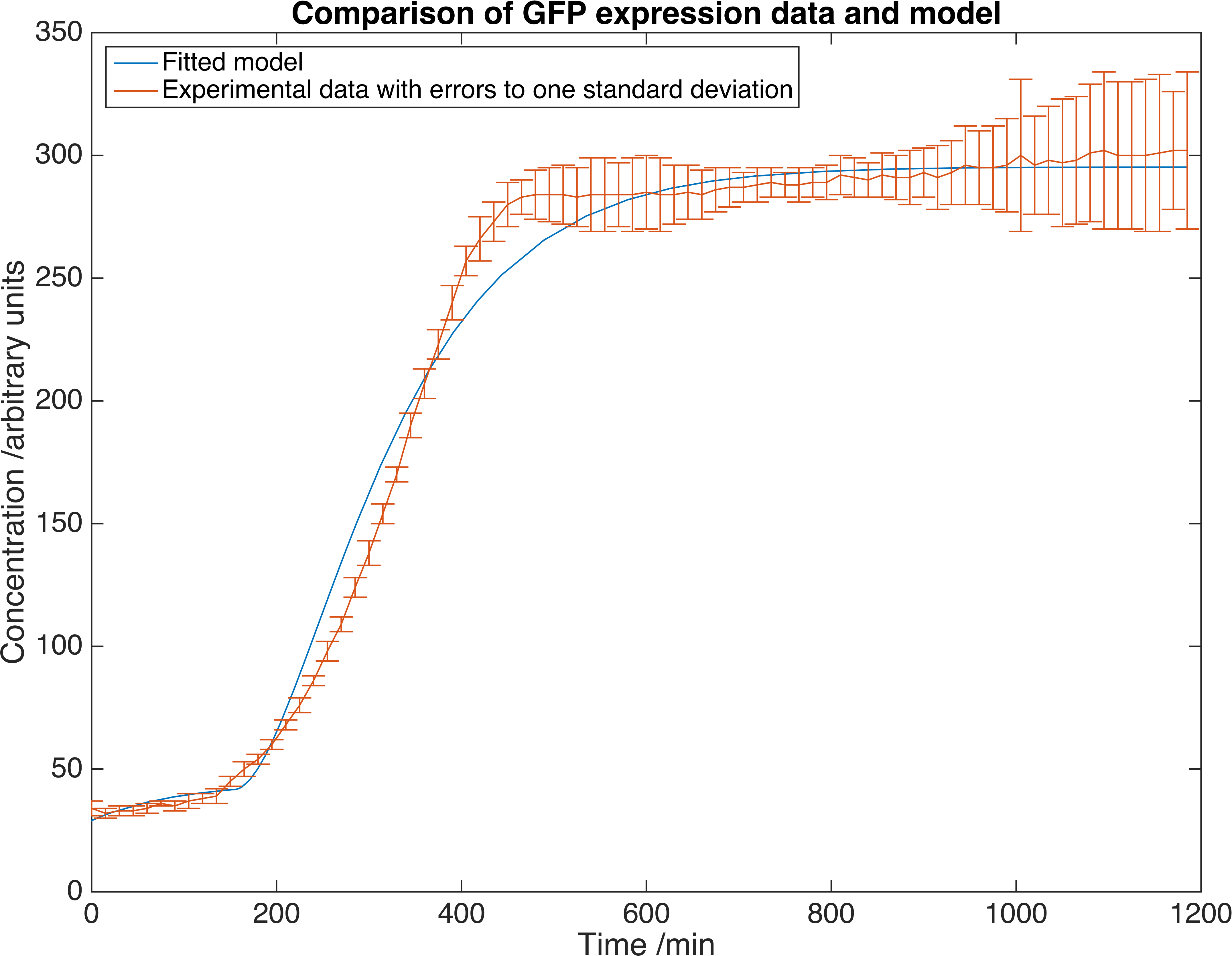
Graph depicting results of GFP concentration as a function of time, matched to our deterministic model. Errors are given to one standard deviation and an arbitrary scaling factor is employed.
By comparing the base-pair length of the GFP gene and of our enzymes, we can expect expression concentrations of the order of \(nM\). This results feeds into our modelling of a mass-exchange system which delivers the enzymes from our cells out to the fluid they're needed in. That model will give us the number of cells required.
Delivery
With the information about the rates of production and concentrations of our products we can look at how the products behave once they leave the cell. This involves modelling the diffusion of the products in different topologies, each associated with a potential physical design of the catheter. With this information we can provide a better estimate of the time scale that our project is working on and assess any need for optimisation.
Dispersin B
Dispersin B is one of the anti-biofilm agents we are using in our project and will be the focus of this delivery section. As such we will assume that conclusions reached apply to all of our enzymes.
A concentration of Dispersin B of 60μg/ml is required to destroy a biofilm that has already formed on a surface. This equates to a concentration of 1.50μM. This is higher than the steady-state gene expression concentration we can expect from our cells, meaning that our system cannot rely solely on diffusion to transport our enzymes to the biofilm. We will therefore model these diffusion systems assuming that our cells are expressing at a 2μM concentration and later we will look at optimising the gene expression to this level.
Beads
Diffusion
The bead delivery system consists of our cells being contained in alginate spheres. Water is passed through the container filled with the beads allowing our enzymes to diffuse from the alginate to the required concentration. More details about the design of the system can be found here.
To determine the convection mass transfer coefficient of Dispersin B from our gel spheres we looked at the diffusion data obtained from this experiment involving the diffusion of crystal violet from our beads. By analysing the system we can produce a theoretical form for the concentration of crystal violet in the bulk water as a function of time:
\[c_{f}=\dfrac{c_{bo}}{1+\frac{V_{f}}{V_{b}}}\left(1-\exp\left(\dfrac{-K_{m}A_{b}\left(1+\frac{V_{f}}{V_{b}}\right)t}{V_{f}}\right)\right)\]| Symbol | Definition | Value | Units |
|---|---|---|---|
| \(A_{b}\) | Total surface area of the beads | \(0.0238\) | \(m^{2}\) |
| \(V_{b}\) | Total volume of beads | \(1.3463\times10^{-5}\) | \(m^{3}\) |
| \(c_{bo}\) | Initial concentration in beads | \(0.02451107\) | \(M\) |
| \(V_{f}\) | Volume of fluid surrounding the beads | \(V_{f}=V_{fo}-\dfrac{1\times10^{-6}}{10}t\) | \(m^{3}\) |
| \(V_{fo}\) | Initial volume of fluid surrounding the beads | \(1\times10^{-4}\) | \(m^{3}\) |
| \(t\) | Time | \(-\) | \(min\) |
| \(c_{f}\) | Concentration of fluid surrounding beads | \(-\) | \(M\) |
| \(K_{m}\) | Convection mass diffusion coefficient | To be fitted | \(mmin^{-1}\) |
The volume of fluid is also a function of time in order to account for the removal of 1ml of water every 10 minutes. The area and volume of the beads is that of 660 spheres with diameter 3.39mm.
However, the number of beads is an estimate. Because of this, in order to fit the curve to the experimental data we must scale the experimental data by an unknown factor. Therefore we preface our equation with an arbitrary scaling factor which, along with the convection diffusion coefficient - \(Km\), is determined by our fitting function.
Our fitting script, detailed here, returned the value of \(K_{m} = 1.7265\times 10^{-5} mmin^{-1}\).
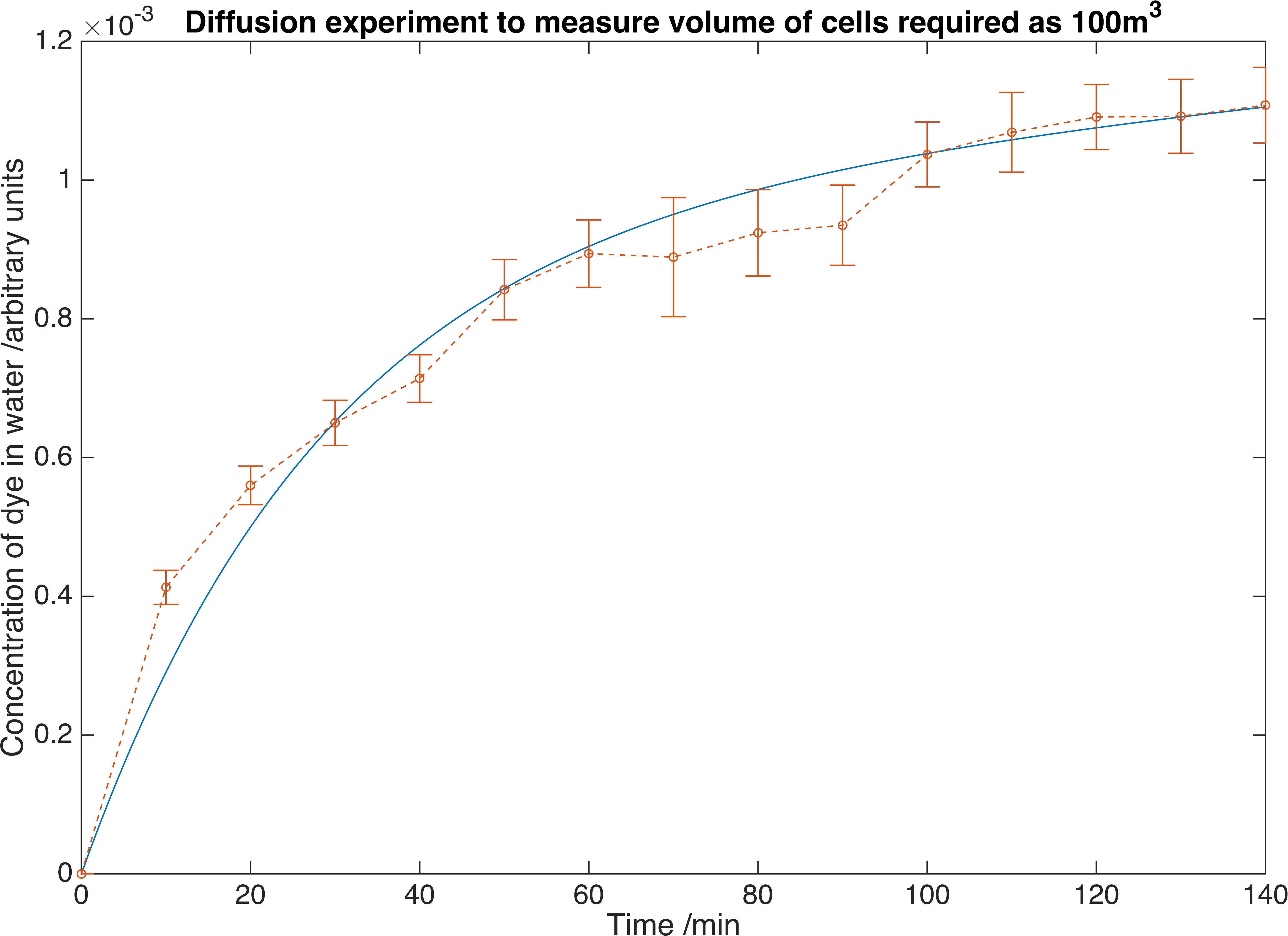
Crystal violet dye diffuses out of alginate beads and concentration is measured. Errors are given to one standard deviation and data is fitted to a deterministic model to determine the mass transfer co-efficient. From this we can determine we would require \(100m^{3}\) of beads to reach the necessary concentration of our own enzymes.
Dispersin B is a significantly larger molecule than crystal violet so this diffusion coefficient will not be close to that for Dispersin B. To correct this we need to make use of similarity. More specifically we take the Sherwood Numbers of the systems to be equal therefore:
\[\left(\dfrac{K_{m}R}{D}\right)_{crystal violet} = \left(\dfrac{K_{m}R}{D}\right)_{Dispersin B}\]| Symbol | Definition | Value | Units |
|---|---|---|---|
| \(D_{crystal violet}\) | Mass diffusivity of crystal violet in water | \(2.8652\times10^{9}\) | \(\mu m^{2}s^{-1}\) |
| \(D_{Dispersin B}\) | Mass diffusivity of Dispersin B in water | \(100\) | \(\mu m^{2}s^{-1}\) |
| \(R\) | Radius of bead | \(1.695\) | \(mm\) |
By rearranging this we arrive at \(\left(K_{m}\right)_{DispersinB} = 6.03\times10^{-13} mmin^{-1}\)
Mass Exchange
This result allows us to theorise a mass exchange system. As a first estimate we will assume that the flow through the beads is sufficiently slow to use the convection diffusion coefficient found above. It is also assumed that the gene expression happens on a faster time scale than the diffusion from the beads to the water, enabling us to assume the concentration of enzyme in the beads remains constant. This is supported by our gene expression models. We can now visualize how the concentrations of the fluid will vary with distance along the mass exchanger:
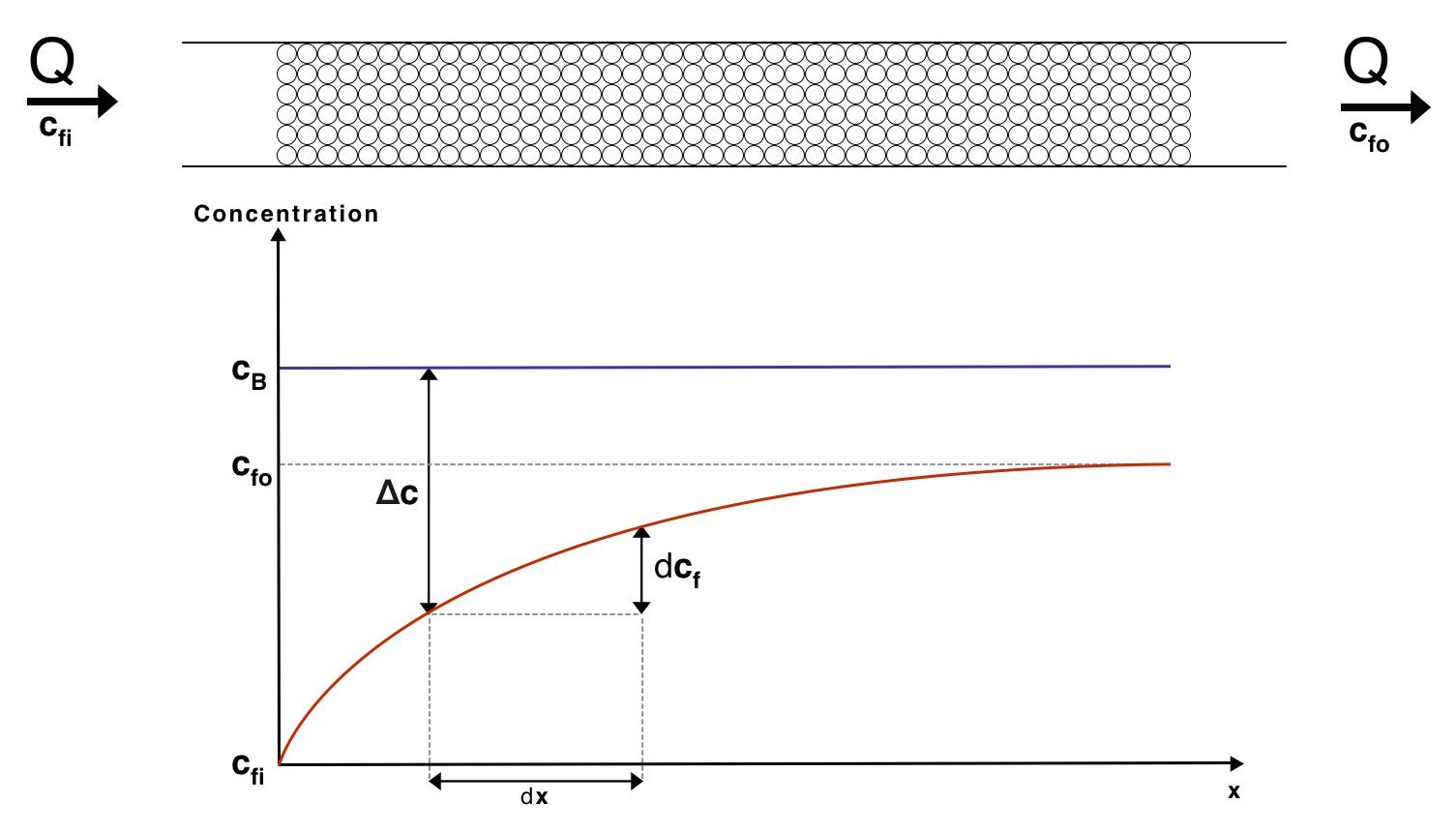
Visualisation of the concentrations of the fluid and the beads along our mass exchanger
The overall system can now be described with the equation:
\[J = K_mA\dfrac{c_{fo}-c_{fi}}{\ln\left(\dfrac{c_{B}-c_{fi}}{c_{B}-c_{fo}}\right)}\]Therefore
\[A = J\dfrac{\ln\left(\dfrac{c_{B}-c_{fi}}{c_{B}-c_{fo}}\right)}{K_{m}\left(c_{fo}-c_{fi}\right)}\]Where \(J=Q\left(c_{fo}-c_{fi}\right)\) and \(Q\) is the volume flow rate of water. We have chosen a flow rate range of 10-100ml/min as this is accepted as a safe artificial bladder fill rate. This range results in the following number of beads required to reach the desired concentration:
Relationship between the number of bacteria-containment beads required to reach a particular flow rate of our enzymes. These are the flow rates we require for practical use.
Therefore a volume of between \(20.3-203m^3\) of beads is required, assuming a packing efficiency of 64%.
However, as stated earlier this estimation relies on the fluid flowing around the beads is slow enough to be approximated as stationary, meaning that mass transfer occurs as natural convection. Although there may be a very large volume of beads and a slow fluid flow rate, the area through which the fluid can flow is likely small enough that the velocity of the fluid is non-negligable.
References