Difference between revisions of "Team:Oxford/Modeling/Tutorial"
| Line 2: | Line 2: | ||
<html> | <html> | ||
| − | <div class="container-fluid page-heading"> | + | <div class="container-fluid page-heading" style="background-image: url(https://static.igem.org/mediawiki/2015/6/6d/Ox_modelling_will_poster.png)"> |
| − | <h3>Modelling</h3> | + | <h3>Modelling Tutorials</h3> |
</div> | </div> | ||
<div class="container-fluid"> | <div class="container-fluid"> | ||
<div class="row"> | <div class="row"> | ||
<div class="col-md-9"> | <div class="col-md-9"> | ||
| − | <div class=" | + | <div class="section" id="introduction"> |
| − | <div class=" | + | <div class="slim"> |
<h2>Introduction</h2> | <h2>Introduction</h2> | ||
<p> | <p> | ||
| − | + | On this page we aim to explain the concepts and methodology behind the <a class="definition" title="model" data-content="A simplified or idealised description of a system or process, usually mathematical, that can be used to predict how it will behave.">model</a>ling we have done in our project. We hope this will make our modelling section more accessible for all members of the iGEM community. | |
| − | + | ||
| − | + | ||
| − | + | ||
| − | + | ||
| − | + | ||
| − | + | ||
</p> | </p> | ||
</div> | </div> | ||
| − | + | </div> | |
| − | + | <div class="section-spacer"></div> | |
| − | <h2>Gene | + | <div class="section" id="gene-expression-networks"> |
| − | + | <div class="slim"> | |
| − | + | <h2>Gene Expression Networks</h2> | |
| − | + | <div id="gene-expression-networks-mass-action"> | |
| − | <div id=" | + | <h3>Mass Action</h3> |
| − | <h3> | + | |
<p> | <p> | ||
| − | + | Our goal is to model a system of reactions such as the reversible reaction | |
</p> | </p> | ||
| + | \[A \mathrel{\mathop{\rightleftharpoons}^{\mathrm{k_{+}}}_{\mathrm{k_{-}}}} B\] | ||
| + | <p> | ||
| + | Where \(A\) and \(B\) are our two species and \(k_{+}\) and \(k_{-}\) will be determined shortly. To do this, we make the intuitive assumption that the rate at which something reacts is proportional to how much of it we've got. That is, the rate of change of \(B\) with time is | ||
| + | </p> | ||
| + | \[\dfrac{dB}{dt}=k_{+}A\] | ||
| + | <p> | ||
| + | where \(k_{+}\) is simply a proportionality constant. This assumption is called the law of mass action. This of course is not the complete picture, as we forgot to include the fact that \(B\) can react back to form \(A\). So the complete system of equations to solve is | ||
| + | </p> | ||
| + | \[\dfrac{dA}{dt}=k_{-}B-k_{+}A\] | ||
| + | \[\dfrac{dB}{dt}=k_{+}A-k_{-}B\] | ||
| + | <p> | ||
| + | At this point, you can type these into your favourite computing program and solve them. | ||
| + | </p> | ||
| + | </div> | ||
| + | <div id="gene-expression-networks-michaelis"> | ||
| + | <h3>Michaelis-Menten Kinetics</h3> | ||
| + | <p> | ||
| + | It is possible to formulate a rate law that describes <a class="definition" title="enzyme" data-content="A molecule which speeds up a chemical reaction - a biological catalyst. The reaction does not involve these molecules.">enzyme</a>-catalysed reactions, this is known as Michaelis-Menten kinetics. In order to derive this rate law we will look at a generalised system of chemical events detailed below: | ||
| + | </p> | ||
| + | |||
| + | \[S + E\mathop{\rightleftharpoons}C_{1}\mathop{\rightleftharpoons}C_{2}\mathop{\rightleftharpoons}P + E\] | ||
| − | \ | + | <p><em> |
| − | + | In this system \(S\) represents our substrate, \(E\) our enzyme, \(C_{1}\) our enzyme-substrate complex, \(C_{2}\) our enzyme-product complex, and \(P\) our product. | |
| + | </em></p> | ||
<p> | <p> | ||
| − | + | Initially we will make two simplifications. Firstly, we will combine \(C_{1}\) and C2 into a single complex, \(C\), as we will assume that the time-scale of the conversion \(C_{1}\mathop{\rightleftharpoons}C_{2}\) is much faster than that of the association and dissociation events. Secondly, we will assume that the product never binds with the free enzyme. These two assumptions lead to the simplified network: | |
</p> | </p> | ||
| + | |||
| + | \[S + E\mathrel{\mathop{\rightleftharpoons}^{k_{1}}_{k_{-1}}}C\mathop{\rightarrow}^{k_{2}}P + E\] | ||
| + | |||
<p> | <p> | ||
| − | + | Using the laws of mass action (detailed above) we arrive at the following differential equation model: | |
</p> | </p> | ||
| + | |||
| + | \[\dfrac{d}{dt}s(t)=-k_{1}s(t)e(t) + k_{-1}c(t)\] | ||
| + | |||
| + | \[\dfrac{d}{dt}e(t)=k_{-1}c(t) - k_{1}s(t)e(t) + k_{2}c(t)\] | ||
| + | |||
| + | \[\dfrac{d}{dt}c(t)=-k_{-1}c(t) + k_{1}s(t)e(t) - k_{2}c(t)\] | ||
| + | |||
| + | \[\dfrac{d}{dt}p(t) = k_{2}c(t)\] | ||
| + | |||
| + | <p><em> | ||
| + | Concentrations are denoted as the lowercase letter eg the concentration of \(S\) is given by \(s\). | ||
| + | </em></p> | ||
| + | |||
<p> | <p> | ||
| − | + | You may have spotted that the enzyme is not consumed in this series of reactions. Therefore the total amount of enzyme remains constant. We reflect this in the expression \(e_{T}=e+c\). We can now use this expression to eliminate \(e(t)\) from our model, leaving: | |
</p> | </p> | ||
| − | + | \[\dfrac{d}{dt}s(t)=-k_{1}s(t)(e_{T}-c(t)) + k_{-1}c(t)\] | |
| + | |||
| + | \[\dfrac{d}{dt}c(t)=-k_{-1}c(t) + k_{1}s(t)(e_{T}-c(t)) - k_{2}c(t)\] | ||
| + | |||
| + | \[\dfrac{d}{dt}p(t) = k_{2}c(t)\] | ||
| − | |||
<p> | <p> | ||
| − | + | We have one further simplification to make. This is the rapid equilibrium approximation, by which we assume that equilibrium between \(s+e\) and \(c\) on a much faster time scale than the reaction of \(c\) to \(p\). With this approximation we can write the following equation: | |
| − | + | ||
| − | + | ||
| − | + | ||
| − | + | ||
| − | + | ||
| − | + | ||
| − | + | ||
| − | + | ||
| − | + | ||
| − | + | ||
| − | + | ||
| − | + | ||
| − | + | ||
| − | + | ||
| − | + | ||
| − | + | ||
| − | + | ||
| − | + | ||
| − | + | ||
| − | + | ||
| − | + | ||
| − | + | ||
| − | + | ||
| − | + | ||
| − | + | ||
| − | + | ||
| − | + | ||
| − | + | ||
| − | + | ||
| − | + | ||
| − | + | ||
| − | + | ||
| − | + | ||
| − | + | ||
| − | + | ||
| − | + | ||
| − | + | ||
| − | + | ||
| − | + | ||
| − | + | ||
| − | + | ||
| − | + | ||
| − | + | ||
| − | + | ||
| − | + | ||
| − | + | ||
| − | + | ||
| − | + | ||
| − | + | ||
| − | + | ||
| − | + | ||
| − | + | ||
| − | + | ||
| − | + | ||
| − | + | ||
| − | + | ||
| − | + | ||
| − | + | ||
| − | + | ||
| − | + | ||
| − | + | ||
| − | + | ||
</p> | </p> | ||
| + | |||
| + | \[0=-k_{-1}c(t) + k_{1}s(t)(e_{T}-c(t)) - k_{2}c(t)\] | ||
| + | |||
<p> | <p> | ||
| − | This | + | Leading to: |
| + | </p> | ||
| + | |||
| + | \[c^{*}(t)= \dfrac{k_{1}s(t)e_{T}}{k_{-1} + k_{2} + k_{1}s(t)}\] | ||
| + | |||
| + | <p> | ||
| + | Now we can see that \(c\) is no longer an independent variable, but instead tracks the other variables. This can be referred to as \(c\) being in quasi-steady state. By including this new expression into our model we are left with: | ||
| + | </p> | ||
| + | |||
| + | \[\dfrac{d}{dt}s(t) = -\dfrac{k_{2}k_{1}s(t)e_{T}}{k_{-1} + k_{2} + k_{1}s(t)}\] | ||
| + | |||
| + | \[\dfrac{d}{dt}p(t) = \dfrac{k_{2}k_{1}s(t)e_{T}}{k_{-1} + k_{2} + k_{1}s(t)}\] | ||
| + | |||
| + | <p> | ||
| + | With this we have an expression describing our enzyme catalysed system in the form of a single reaction. The rate of this reaction is known as a Michaelis-Menten rate law. By defining \(K_{max}=k_{2}e_{T}\) and \(K_{half}=\dfrac{k_{-1}+k_{2}}{k_{1}}\) we can express in the more familiar form: | ||
| + | </p> | ||
| + | |||
| + | \[rate \: of \: S \mathop{\rightarrow} P = K_{max}\dfrac{s}{K_{half} + s}\] | ||
| + | |||
| + | <p> | ||
| + | It is worth noting that there are a number of ways to derive this form, each involving different approximations. These methods may lead to the constants \(K_{max}\) and \(K_{half}\) being defined differently. | ||
| + | </p> | ||
| + | |||
| + | </div> | ||
| + | <div id="gene-expression-networks-stochastic"> | ||
| + | <h3>Stochastic modelling</h3> | ||
| + | <p> | ||
| + | In our project we experimented with stochastic models to evaluate gene expression parameters, much like the deterministic models above. We ran the model here but found that it was not directly insightful to the project, so it has been relegated to the tutorials section. | ||
| + | </p> | ||
| + | <p> | ||
| + | The simplest way to add an element of 'randomness' into an equation is to add a random term into the differential equation. This turns it into a <a class="definition" title="stochastic" data-content="A stochastic model predicts a set of possible outcomes weighted by their likelihoods, or probabilities. It allows for an element of randomness.">stochastic</a> differential equation, such as: | ||
| + | </p> | ||
| + | \[\dfrac{dx}{dt}=c+r\] | ||
| + | <div class="image image-right"> | ||
| + | <img src="https://static.igem.org/mediawiki/2015/1/1f/OxiGEM_Stochastic_Tutorial_01.jpg"/> | ||
| + | </div> | ||
| + | <p> | ||
| + | which determines the evolution of a particle travelling at a speed \(c\), with a random number \(r\) added into the mix just for fun. We choose \(r\) to be normally distributed with a mean value of 0 and a variance of, say, 1. We evaluate the position of the particle at multiple timesteps (with some small time \(dt\) separating them) and plot our solution in the Figure below. | ||
| + | </p> | ||
| + | <p> | ||
| + | We can do better than this when dealing with systems such as our example in the previous section. We use the Gillespie algorithm to find: | ||
| + | </p> | ||
| + | <ol> | ||
| + | <li>The <strong>time</strong> taken between reactions</li> | ||
| + | <li>The <strong>reaction</strong> that took place in that time.</li> | ||
| + | </ol> | ||
| + | <p> | ||
| + | as neither of these could be determined by our initial method [<a href="#Ref2">2</a>, <a href="#Ref4">4</a>]. | ||
</p> | </p> | ||
<div class="image image-full"> | <div class="image image-full"> | ||
| − | <img src="https://static.igem.org/mediawiki/2015/ | + | <img src="https://static.igem.org/mediawiki/2015/7/72/OxiGEM_Stochastic_Tutorial_02.png"/> |
| − | + | ||
| − | + | ||
| − | + | ||
</div> | </div> | ||
<p> | <p> | ||
| − | We | + | <strong>1)</strong> To find the time taken, we make an assumption about the form of the probability distribution that the time between reactions holds. It makes sense to think of it as a falling exponential, such that reactions more often happen quickly rather than slowly, and that the more probable a reaction is, the shorter the time between subsequent reactions. This naturally leads to the form |
| + | </p> | ||
| + | \[P(t)=e^{-\alpha_{0}t}\] | ||
| + | <p> | ||
| + | where \(P(t)\) is the probability of any reaction occuring in time \(t\), and \(\alpha_{0}\) tells us something about the likelihood of the reaction. We plot this in the Figure. In fact we call \(\alpha_{0}\) the sum of the propensities \(\alpha_{i}\) (where the dummy variable \(i\) runs from 1 to the number of possible reactions, \(N\), that could occur). In the case of our example system, the propensity for the reaction \(A\) to \(B\) would be \(k_{+}A\) and the propensity for the reaction \(B\) to \(A\) is \(k_{-}B\) so in this case \(\alpha_{0}=k_{+}A+k_{-}B\). | ||
| + | </p> | ||
| + | <p> | ||
| + | To decide the time it took for a reaction to occur, we sample a random number \(r_{1}\) in the range [0,1] and stick that number on the y axis of the graph. We read off from our graph a corresponding time and we're done - we now know when the next reaction took place. | ||
</p> | </p> | ||
| − | |||
| − | |||
| − | |||
| − | |||
| − | |||
| − | |||
| − | |||
| − | |||
| − | |||
| − | |||
| − | |||
| − | |||
| − | |||
| − | |||
| − | |||
| − | |||
| − | |||
| − | |||
| − | |||
| − | |||
| − | |||
| − | |||
| − | |||
| − | |||
| − | |||
| − | |||
| − | |||
| − | |||
| − | |||
| − | |||
| − | |||
| − | |||
| − | |||
| − | |||
| − | |||
| − | |||
| − | |||
| − | |||
| − | |||
| − | |||
| − | |||
| − | |||
| − | |||
| − | |||
| − | |||
| − | |||
| − | |||
| − | |||
| − | |||
| − | |||
| − | |||
| − | |||
| − | |||
| − | |||
| − | |||
| − | |||
| − | |||
| − | |||
| − | |||
| − | |||
| − | |||
| − | |||
| − | |||
| − | |||
| − | |||
| − | |||
| − | |||
| − | |||
| − | |||
| − | |||
| − | |||
| − | |||
| − | |||
| − | |||
| − | |||
| − | |||
<p> | <p> | ||
| − | + | <strong>2)</strong> To decide which reaction took place, we need the probabilities of each reaction occuring being proportional to the ratio of their propensities. We split up the domain of 0 to 1 into the normalised ratios of the propensities of our problem, recalling the propensities we calculated. We could have, in this case, selected the backwards reaction B to A. We can generalise this to the form given in the Gillespie Algorithm above. | |
</p> | </p> | ||
<div class="image image-full"> | <div class="image image-full"> | ||
| − | <img src="https://static.igem.org/mediawiki/2015/ | + | <img src="https://static.igem.org/mediawiki/2015/d/da/OxiGEM_Stochastic_Tutorial_03.jpg"/> |
| − | + | ||
| − | + | ||
| − | + | ||
</div> | </div> | ||
<p> | <p> | ||
| − | + | We have also produced a video tutorial on the subject, which you can watch below. | |
</p> | </p> | ||
</div> | </div> | ||
</div> | </div> | ||
| + | <video class="image-massive" poster="https://static.igem.org/mediawiki/2015/6/6d/Ox_modelling_will_poster.png" controls> | ||
| + | <source src="https://static.igem.org/mediawiki/2015/b/b2/OxiGEM_Modelling_With_Will.mp4" type="video/mp4"> | ||
| + | Your browser does not support the video tag. | ||
| + | </video> | ||
</div> | </div> | ||
| − | <div class=" | + | <div class="section-spacer"></div> |
| − | + | <div class="section" id="diffusion"> | |
| − | + | <div class="slim"> | |
| − | <div class=" | + | <h2>Diffusion</h2> |
| − | <div class=" | + | |
| − | <h2> | + | |
<p> | <p> | ||
| − | + | In this section we will derive some of the equations used in the <a href="https://2015.igem.org/Team:Oxford/Modeling#delivery">Delivery Section</a>. | |
</p> | </p> | ||
| − | <div id=" | + | <div id="diffusion-beads"> |
| − | <h3> | + | <h3>Diffusion out of our Beads</h3> |
<p> | <p> | ||
| − | + | In order to find the convection mass transfer coefficient, \(K_m\) of our beads in water we needed derive a theoretical curve to fit our experimental data to. To do this, we made a number of approximations. Our beads are assumed to be spherical and of the diameter. We also used a lumped capacitance model, in which the concentration of substance is assumed to be uniform within the bead. We will also make use of the equivalence of heat and mass transfer. | |
</p> | </p> | ||
<p> | <p> | ||
| − | + | Our derivation starts from Newton's law of cooling | |
</p> | </p> | ||
| − | |||
| − | |||
| − | |||
| − | |||
| − | |||
| − | |||
| − | |||
| − | |||
| − | |||
| − | |||
| − | |||
| − | + | \[Q = hA\Delta T\] | |
| − | + | <p> | |
| − | + | Where \(Q\) is the flow of energy, \(h\) is the convection coefficient, and \(\Delta T\) is the difference in temperature accross the boundary. Or rather its mass equivalent | |
| − | + | </p> | |
| − | + | \[\dot{m}=K_{m}A_{b}\left(c_{b}-c_{f}\right)\] | |
| − | + | <p> | |
| − | + | Where the mass flow rate, \(\dot{m}\), across a boundary is driven by the concentration difference across it. In our case the concentration difference is between the concentration of particles, \(c_f\) in the fluid and the beads, \(c_b\). Using the relationship | |
| − | + | </p> | |
| − | + | \[\dot{m}=V_{f}\dot{c_{f}}=-V_{b}\dot{c_{b}}\] | |
| − | + | <p> | |
| − | + | With \(V_f\) and \(c_f\) as the concentration and volume of the fluid surrounding the beads, as well as \(A\), \(V_b\) and \(c_b\) representing the total area, volume and concentration of the beads themselves. We arrive at | |
| − | + | </p> | |
| − | + | ||
| − | + | ||
| − | + | ||
| − | + | ||
| − | + | ||
| − | + | ||
| − | + | ||
| − | + | ||
| − | + | ||
| − | + | ||
| − | + | ||
| − | + | ||
| − | + | ||
| − | + | ||
| − | + | ||
| − | + | ||
| − | + | ||
| − | + | ||
| − | + | ||
| − | + | ||
| − | + | ||
| − | + | ||
| − | + | ||
| − | + | ||
| − | + | ||
| − | + | ||
| − | + | ||
| − | + | ||
| − | + | ||
| − | + | ||
| − | + | ||
| − | + | ||
| − | + | ||
| − | + | ||
| − | + | ||
| − | + | ||
| − | + | ||
| − | + | ||
| − | + | ||
| − | + | ||
| − | + | ||
| − | + | ||
| − | + | ||
| − | + | ||
| − | + | ||
| − | + | ||
| − | + | ||
| − | + | ||
| − | + | ||
| − | + | ||
| − | + | ||
| − | + | ||
| − | + | ||
| − | + | ||
| − | + | ||
| − | + | ||
| − | + | ||
| − | + | ||
| − | + | ||
| − | + | ||
| − | + | ||
| − | + | ||
| − | + | ||
| − | + | \[\dot{c_{b}}=-\dfrac{V_{f}}{V_{b}}\dot{c_{f}}\quad c_{b}=c_{bo}-\dfrac{V_{f}}{V_{b}}c_{f}\] | |
| − | + | <p> | |
| − | + | In this \(c_{b0}\) is the initial concentration of the beads. By substituting this into the mass equivalent of Newton's law of cooling we arrive at the expression | |
| − | + | </p> | |
| − | + | \[V_{f}\dot{c_{f}}=K_{m}A_{b}\left(c_{bo}-\left(1+\dfrac{V_{f}}{V_{b}}\right)c_{f}\right)\] | |
| − | + | <p> | |
| − | + | This expression can be rearranged and integrated to with respect to time to give | |
| − | + | </p> | |
| − | + | \[c_{f}=\dfrac{c_{bo}}{\left(1+\frac{V_{f}}{V_{b}}\right)}-\dfrac{V_{f}}{K_{m}A_{b}\left(1+\frac{V_{f}}{V_{b}}\right)}\exp\left(-\dfrac{K_{m}A_{b}\left(1+\frac{V_{f}}{V_{b}}\right)\left(t+k\right)}{V_{f}}\right)\] | |
| − | + | <p> | |
| − | + | where \(k\) constant that comes from integration. | |
| − | + | </p> | |
| − | + | <p> | |
| − | + | At \(t=0\) \(c_f=0\), leaving us with | |
| − | + | </p> | |
| − | + | \[\dfrac{c_{bo}}{\left(1+\frac{V_{f}}{V_{b}}\right)}=\dfrac{V_{f}}{K_{m}A_{b}\left(1+\frac{V_{f}}{V_{b}}\right)}\exp\left(-\dfrac{K_{m}A_{b}\left(1+\frac{V_{f}}{V_{b}}\right)k}{V_{f}}\right)\] | |
| − | + | <p> | |
| − | + | resulting in | |
| − | + | </p> | |
| − | + | \[k=-\dfrac{V_{f}}{K_{m}A_{b}\left(1+\frac{V_{f}}{V_{b}}\right)}\ln\left(\dfrac{K_{m}A_{b}c_{bo}}{V_{f}}\right)\] | |
| − | + | <p> | |
| − | + | and therefore | |
| − | + | </p> | |
| − | + | \[c_{f}=\dfrac{c_{bo}}{1+\frac{V_{f}}{V_{b}}}\left(1-\exp\left(-\dfrac{K_{m}A_{b}\left(1+\frac{V_{f}}{V_{b}}\right)}{V_{f}}t\right)\right)\] | |
| − | + | <p> | |
| − | + | This shows how the concentration of fluid varies over time when there is a constant volume of fluid surrounding the beads. However, in the experiment, 1ml of water was removed every 10 minutes. We account for this by taking \(V_f=V_{fo}-\dfrac{1\times10^{-6}}{10}\). Where volumes are given in \(m^3\), time is in minutes and \(V_fo\) is the initial volume of the fluid surrounding the beads. | |
| − | + | </p> | |
| − | + | <p> | |
| − | + | Now we have derived the final expression, have a look at how this result was fitted to the experimental data to determine the value of \(K_m\) <a href="https://2015.igem.org/Team:Oxford/Modeling#delivery-beads-diffusion">here</a>. | |
| − | + | </p> | |
| − | + | </div> | |
| − | + | <div id="diffusion-mass-exchanger"> | |
| − | + | <h3>Mass Exchanger</h3> | |
| − | + | <p> | |
| − | + | In our analysis of the use of beads in a mass exchange system we used the expression | |
| − | + | </p> | |
| − | + | \[J = K_mA\dfrac{c_{fo}-c_{fi}}{\ln\left(\dfrac{c_{B}-c_{fi}}{c_{B}-c_{fo}}\right)}\] | |
| − | + | <p> | |
| − | + | but where did this come from? | |
| − | + | </p> | |
| − | + | <p> | |
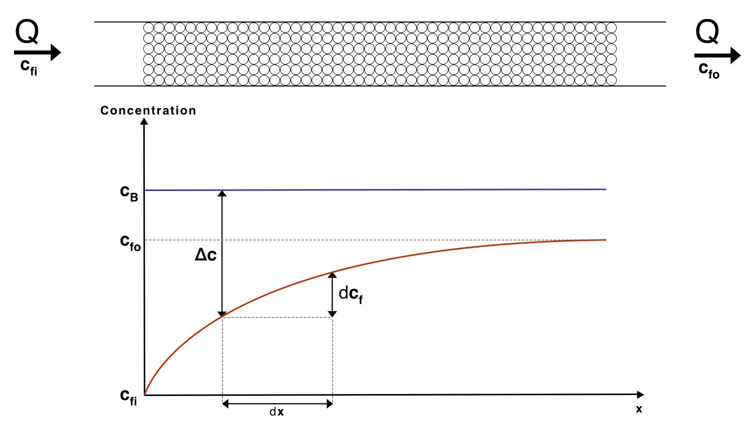
| − | + | For this derivation we need to take a look at the mass flow out of the beads across a differential area, \(dA\). To help visulise the system below is a diagram showing how the conentration of proteins varies through the mass exchanger. | |
| − | + | </p> | |
| − | + | <div class="image image-full"> | |
| − | + | <img src="https://static.igem.org/mediawiki/2015/e/e0/Ox_mass_exchange_daig.jpg"/> | |
| − | + | ||
| − | + | ||
| − | + | ||
| − | + | ||
| − | + | ||
| − | + | ||
| − | + | ||
| − | + | ||
| − | + | ||
| − | + | ||
| − | + | ||
| − | + | ||
| − | + | ||
| − | + | ||
| − | + | ||
| − | + | ||
| − | + | ||
| − | + | ||
| − | + | ||
| − | + | ||
| − | + | ||
| − | + | ||
| − | + | ||
| − | + | ||
| − | + | ||
| − | + | ||
| − | + | ||
| − | + | ||
| − | + | ||
| − | + | ||
| − | + | ||
| − | + | ||
| − | + | ||
| − | + | ||
| − | + | ||
| − | + | ||
| − | + | ||
| − | + | ||
| − | + | ||
| − | + | ||
| − | + | ||
| − | + | ||
| − | + | ||
| − | + | ||
| − | + | ||
| − | + | ||
</div> | </div> | ||
| + | <p> | ||
| + | The mass flow rate across a differential area, \(dJ\) can be expressed as | ||
| + | </p> | ||
| + | \[dJ=K_{m}\left(c_{B}-c_{f}\right)dA\] | ||
| + | <p> | ||
| + | This expression comes from the mass equivalent of Newton's law of cooling. We may use the relationship | ||
| + | </p> | ||
| + | \[dJ=Qdc_{f}\] | ||
| + | <p> | ||
| + | Where \(Q\) is the volume flow rate of water through the mass exchanger. By combining these 2 relationships we arrive at | ||
| + | </p> | ||
| + | \[d\Delta c=-\dfrac{dJ}{Q}=\dfrac{-K_{m}\left(\Delta c\right)dA}{Q}\] | ||
| + | \[d\Delta c=\dfrac{-K_{m}\left(\Delta c\right)dA}{Q}\] | ||
| + | <p> | ||
| + | In this expression \(\Delta c=c_b-c_f\) at a distance \(x\) from the start of the mass exchanger. Rearranging and integrating leads to | ||
| + | </p> | ||
| + | \[\ln\left(\dfrac{\Delta c_{i}}{\Delta c_{o}}\right)=\dfrac{K_{m}}{Q}A\] | ||
| + | <p> | ||
| + | Where \(\Delta c_{i}\) and \(\Delta c_{o}\) are the concentration differences at the inlet and outlet of the mass exchanger respectively. Thus \(\Delta c_{i} = c_B - c_{fi}\) and \(\Delta c_{o} = c_B - c_{fo}\). | ||
| + | </p> | ||
| + | <p> | ||
| + | The total mass flow, \(J\), can also be expressed as \(J=Q\left(c_{fo}-c_{fi}\right)\). Substituting this into the previous expression gives us | ||
| + | </p> | ||
| + | \[\ln\left(\dfrac{\Delta c_{i}}{\Delta c_{o}}\right)=\dfrac{K_{m}A\left(c_{fo}-c_{fi}\right)}{J}\] | ||
| + | <p> | ||
| + | Which can be rearranged into the form | ||
| + | </p> | ||
| + | \[J=K_{m}A\dfrac{\left(c_{fo}-c_{fi}\right)}{\ln\left(\dfrac{c_{B}-c_{fi}}{c_{B}-c_{fo}}\right)}\] | ||
| + | <p> | ||
| + | Comparing this to the form of the mass equivalent of Newton's law of cooling, \(J = K_mA\Delta c\), we see that we have derived an effective average concentration difference across the entire mass exchanger. This is known as the log mean concentration difference. We used this result to determine an estimate for the total exchange area required for our system, <a href="https://2015.igem.org/Team:Oxford/Modeling#delivery-beads-mass-exchange">here</a>. | ||
| + | </p> | ||
</div> | </div> | ||
| − | |||
| − | |||
| − | |||
| − | |||
| − | |||
| − | |||
| − | |||
| − | |||
</div> | </div> | ||
| + | </div> | ||
| + | <div class="section-spacer"> | ||
| + | </div> | ||
| + | <div class="section" id="stochastic-diffusion"> | ||
| + | <h2> Stochastic Diffusion </h2> | ||
| + | <p> | ||
| + | We explored a stochastic diffusion model in our project. We used it to find the time taken for our enzymes to diffuse from the outer radius of the catheter into its centre. This information does not inform much about the design of the project, but the modelling is interesting and may be useful for future iGEM teams. | ||
| + | </p> | ||
| + | <p> | ||
| + | We consider a number of particles that start at some initial location. In our case, this is the outer edge of the circle that represents the cross section of the catheter. The evolution of each particle is then given by the stochastic differential equations | ||
| + | </p> | ||
| + | \[X(t+\triangle t)=X(t)+\sqrt{2D\triangle t}\xi_{r}\cos\theta | ||
| + | \] | ||
| + | \[Y(t+\triangle t)=Y(t)+\sqrt{2D\triangle t}\xi_{r}\sin\theta | ||
| + | \] | ||
| + | <p> | ||
| + | Where \(X\) and \(Y\) represent the spatial coordinates of the particle as functions of time, \(D\) is the diffusion constant, \(\triangle t\) is the time size of the time step, \(\xi_{r}\) is a random number taken from the normal distribution with mean 0 and variance 1, and \(\theta \) is an angle taken from a uniform probability distribution in the range \([0,2\pi ]\). We find new random numbers \(\xi_{r}\) and \(\theta \) for each time step \(\triangle t\) and for each particle. | ||
| + | </p> | ||
| + | <p> | ||
| + | Below, we run the simulation for a typical catheter (with a diameter of 5mm []) that initially houses fifty proteins at each point on its rim. We take the diffusion constant to be \(10^{-4}mm^{2}sec^{-1} [], \(\triangle t\) to be one second, and record a video of the result. Each frame represents one second and there are ten frames per second. The x and y axes represent position (scaled such that the whole ring is of diameter 5mm) and the z axis represents the absolute number of particles at that position, where each tick represents two particles. | ||
| + | </p> | ||
| + | </div> | ||
| + | <video class="image-massive" controls> | ||
| + | <source src="https://static.igem.org/mediawiki/2015/5/58/OxiGEM_Ring_Diffusion_Video.mp4" type="video/mp4"> | ||
| + | Your browser does not support the video tag. | ||
| + | </video> | ||
| + | <div class="section"> | ||
| + | <p> | ||
| + | We conclude that the time taken for the centre of the catheter to reach a concentration >60% of the outer rim is of the order of 5 minutes. This means that we would not need to consider optimising our design because of this effect. The model can be easily adapted to a space with a different shape. | ||
| + | </p> | ||
</div> | </div> | ||
<div class="section" id="references"> | <div class="section" id="references"> | ||
| − | |||
<ol class="references"> | <ol class="references"> | ||
| − | <li> | + | <li>Brian Ingalls, Mathematical Modeling in Systems Biology: An Introduction, 2012 University of Waterloo</li> |
| − | + | <li>R. Erban, S. J. Chapman, and P. Maini. A practical guide to stochastic simulations of reaction- diffusion processes, 2007. Available <a href="http://arxiv.org/abs/0704.1908">here</a><a name="Ref2"></a></li> | |
| − | <li><a href="http:// | + | <li><a href="https://www.cpp.edu/~tknguyen/che313/pdf/chap3-1.pdf">https://www.cpp.edu/~tknguyen/che313/pdf/chap3-1.pdf</a></li> |
| − | + | ||
| − | + | ||
| − | + | ||
| − | <li> | + | |
| − | + | ||
| − | + | ||
| − | + | ||
| − | + | ||
| − | + | ||
| − | + | ||
| − | + | ||
| − | + | ||
| − | + | ||
| − | + | ||
</ol> | </ol> | ||
</div> | </div> | ||
</div> | </div> | ||
<div class="col-md-3 contents-sidebar"> | <div class="col-md-3 contents-sidebar"> | ||
| − | <ul id="sidebar" class="nav nav-stacked | + | <ul id="sidebar" class="nav nav-stacked" data-spy="affix"> |
| − | <li> | + | <li><a href="#introduction">Introduction</a></li> |
| − | + | ||
| − | + | ||
<li> | <li> | ||
| − | <a href="# | + | <a href="#gene-expression-networks">Gene Expression Networks</a> |
<ul class="nav nav-stacked"> | <ul class="nav nav-stacked"> | ||
| − | <li><a href="# | + | <li><a href="#gene-expression-networks-mass-action">Mass Action</a></li> |
| + | <li><a href="#gene-expression-networks-michaelis">Michaelis-Menten Kinetics</a></li> | ||
| + | <li><a href="#gene-expression-networks-stochastic">Stochastic</a></li> | ||
</ul> | </ul> | ||
</li> | </li> | ||
<li> | <li> | ||
| − | <a href="# | + | <a href="#diffusion">Deterministic Diffusion</a> |
<ul class="nav nav-stacked"> | <ul class="nav nav-stacked"> | ||
| − | <li><a href="# | + | <li><a href="#diffusion-beads">Diffusion out of our Beads</a></li> |
| − | <li> | + | <li><a href="#diffusion-mass-exchanger">Mass Exchanger</a></li> |
| − | + | ||
| − | + | ||
| − | + | ||
| − | + | ||
| − | + | ||
| − | + | ||
</ul> | </ul> | ||
| − | <a href=" | + | </li> |
| + | <li> | ||
| + | <a href="stochastic-diffusion">Stochastic Diffusion</a> | ||
</li> | </li> | ||
<li> | <li> | ||
<a href="#references">References</a> | <a href="#references">References</a> | ||
</li> | </li> | ||
| + | |||
</ul> | </ul> | ||
</div> | </div> | ||
Revision as of 16:06, 18 September 2015
Modelling Tutorials
Introduction
On this page we aim to explain the concepts and methodology behind the modelling we have done in our project. We hope this will make our modelling section more accessible for all members of the iGEM community.
Gene Expression Networks
Mass Action
Our goal is to model a system of reactions such as the reversible reaction
\[A \mathrel{\mathop{\rightleftharpoons}^{\mathrm{k_{+}}}_{\mathrm{k_{-}}}} B\]Where \(A\) and \(B\) are our two species and \(k_{+}\) and \(k_{-}\) will be determined shortly. To do this, we make the intuitive assumption that the rate at which something reacts is proportional to how much of it we've got. That is, the rate of change of \(B\) with time is
\[\dfrac{dB}{dt}=k_{+}A\]where \(k_{+}\) is simply a proportionality constant. This assumption is called the law of mass action. This of course is not the complete picture, as we forgot to include the fact that \(B\) can react back to form \(A\). So the complete system of equations to solve is
\[\dfrac{dA}{dt}=k_{-}B-k_{+}A\] \[\dfrac{dB}{dt}=k_{+}A-k_{-}B\]At this point, you can type these into your favourite computing program and solve them.
Michaelis-Menten Kinetics
It is possible to formulate a rate law that describes enzyme-catalysed reactions, this is known as Michaelis-Menten kinetics. In order to derive this rate law we will look at a generalised system of chemical events detailed below:
\[S + E\mathop{\rightleftharpoons}C_{1}\mathop{\rightleftharpoons}C_{2}\mathop{\rightleftharpoons}P + E\]In this system \(S\) represents our substrate, \(E\) our enzyme, \(C_{1}\) our enzyme-substrate complex, \(C_{2}\) our enzyme-product complex, and \(P\) our product.
Initially we will make two simplifications. Firstly, we will combine \(C_{1}\) and C2 into a single complex, \(C\), as we will assume that the time-scale of the conversion \(C_{1}\mathop{\rightleftharpoons}C_{2}\) is much faster than that of the association and dissociation events. Secondly, we will assume that the product never binds with the free enzyme. These two assumptions lead to the simplified network:
\[S + E\mathrel{\mathop{\rightleftharpoons}^{k_{1}}_{k_{-1}}}C\mathop{\rightarrow}^{k_{2}}P + E\]Using the laws of mass action (detailed above) we arrive at the following differential equation model:
\[\dfrac{d}{dt}s(t)=-k_{1}s(t)e(t) + k_{-1}c(t)\] \[\dfrac{d}{dt}e(t)=k_{-1}c(t) - k_{1}s(t)e(t) + k_{2}c(t)\] \[\dfrac{d}{dt}c(t)=-k_{-1}c(t) + k_{1}s(t)e(t) - k_{2}c(t)\] \[\dfrac{d}{dt}p(t) = k_{2}c(t)\]Concentrations are denoted as the lowercase letter eg the concentration of \(S\) is given by \(s\).
You may have spotted that the enzyme is not consumed in this series of reactions. Therefore the total amount of enzyme remains constant. We reflect this in the expression \(e_{T}=e+c\). We can now use this expression to eliminate \(e(t)\) from our model, leaving:
\[\dfrac{d}{dt}s(t)=-k_{1}s(t)(e_{T}-c(t)) + k_{-1}c(t)\] \[\dfrac{d}{dt}c(t)=-k_{-1}c(t) + k_{1}s(t)(e_{T}-c(t)) - k_{2}c(t)\] \[\dfrac{d}{dt}p(t) = k_{2}c(t)\]We have one further simplification to make. This is the rapid equilibrium approximation, by which we assume that equilibrium between \(s+e\) and \(c\) on a much faster time scale than the reaction of \(c\) to \(p\). With this approximation we can write the following equation:
\[0=-k_{-1}c(t) + k_{1}s(t)(e_{T}-c(t)) - k_{2}c(t)\]Leading to:
\[c^{*}(t)= \dfrac{k_{1}s(t)e_{T}}{k_{-1} + k_{2} + k_{1}s(t)}\]Now we can see that \(c\) is no longer an independent variable, but instead tracks the other variables. This can be referred to as \(c\) being in quasi-steady state. By including this new expression into our model we are left with:
\[\dfrac{d}{dt}s(t) = -\dfrac{k_{2}k_{1}s(t)e_{T}}{k_{-1} + k_{2} + k_{1}s(t)}\] \[\dfrac{d}{dt}p(t) = \dfrac{k_{2}k_{1}s(t)e_{T}}{k_{-1} + k_{2} + k_{1}s(t)}\]With this we have an expression describing our enzyme catalysed system in the form of a single reaction. The rate of this reaction is known as a Michaelis-Menten rate law. By defining \(K_{max}=k_{2}e_{T}\) and \(K_{half}=\dfrac{k_{-1}+k_{2}}{k_{1}}\) we can express in the more familiar form:
\[rate \: of \: S \mathop{\rightarrow} P = K_{max}\dfrac{s}{K_{half} + s}\]It is worth noting that there are a number of ways to derive this form, each involving different approximations. These methods may lead to the constants \(K_{max}\) and \(K_{half}\) being defined differently.
Stochastic modelling
In our project we experimented with stochastic models to evaluate gene expression parameters, much like the deterministic models above. We ran the model here but found that it was not directly insightful to the project, so it has been relegated to the tutorials section.
The simplest way to add an element of 'randomness' into an equation is to add a random term into the differential equation. This turns it into a stochastic differential equation, such as:
\[\dfrac{dx}{dt}=c+r\]
which determines the evolution of a particle travelling at a speed \(c\), with a random number \(r\) added into the mix just for fun. We choose \(r\) to be normally distributed with a mean value of 0 and a variance of, say, 1. We evaluate the position of the particle at multiple timesteps (with some small time \(dt\) separating them) and plot our solution in the Figure below.
We can do better than this when dealing with systems such as our example in the previous section. We use the Gillespie algorithm to find:
- The time taken between reactions
- The reaction that took place in that time.
as neither of these could be determined by our initial method [2, 4].

1) To find the time taken, we make an assumption about the form of the probability distribution that the time between reactions holds. It makes sense to think of it as a falling exponential, such that reactions more often happen quickly rather than slowly, and that the more probable a reaction is, the shorter the time between subsequent reactions. This naturally leads to the form
\[P(t)=e^{-\alpha_{0}t}\]where \(P(t)\) is the probability of any reaction occuring in time \(t\), and \(\alpha_{0}\) tells us something about the likelihood of the reaction. We plot this in the Figure. In fact we call \(\alpha_{0}\) the sum of the propensities \(\alpha_{i}\) (where the dummy variable \(i\) runs from 1 to the number of possible reactions, \(N\), that could occur). In the case of our example system, the propensity for the reaction \(A\) to \(B\) would be \(k_{+}A\) and the propensity for the reaction \(B\) to \(A\) is \(k_{-}B\) so in this case \(\alpha_{0}=k_{+}A+k_{-}B\).
To decide the time it took for a reaction to occur, we sample a random number \(r_{1}\) in the range [0,1] and stick that number on the y axis of the graph. We read off from our graph a corresponding time and we're done - we now know when the next reaction took place.
2) To decide which reaction took place, we need the probabilities of each reaction occuring being proportional to the ratio of their propensities. We split up the domain of 0 to 1 into the normalised ratios of the propensities of our problem, recalling the propensities we calculated. We could have, in this case, selected the backwards reaction B to A. We can generalise this to the form given in the Gillespie Algorithm above.

We have also produced a video tutorial on the subject, which you can watch below.
Diffusion
In this section we will derive some of the equations used in the Delivery Section.
Diffusion out of our Beads
In order to find the convection mass transfer coefficient, \(K_m\) of our beads in water we needed derive a theoretical curve to fit our experimental data to. To do this, we made a number of approximations. Our beads are assumed to be spherical and of the diameter. We also used a lumped capacitance model, in which the concentration of substance is assumed to be uniform within the bead. We will also make use of the equivalence of heat and mass transfer.
Our derivation starts from Newton's law of cooling
\[Q = hA\Delta T\]Where \(Q\) is the flow of energy, \(h\) is the convection coefficient, and \(\Delta T\) is the difference in temperature accross the boundary. Or rather its mass equivalent
\[\dot{m}=K_{m}A_{b}\left(c_{b}-c_{f}\right)\]Where the mass flow rate, \(\dot{m}\), across a boundary is driven by the concentration difference across it. In our case the concentration difference is between the concentration of particles, \(c_f\) in the fluid and the beads, \(c_b\). Using the relationship
\[\dot{m}=V_{f}\dot{c_{f}}=-V_{b}\dot{c_{b}}\]With \(V_f\) and \(c_f\) as the concentration and volume of the fluid surrounding the beads, as well as \(A\), \(V_b\) and \(c_b\) representing the total area, volume and concentration of the beads themselves. We arrive at
\[\dot{c_{b}}=-\dfrac{V_{f}}{V_{b}}\dot{c_{f}}\quad c_{b}=c_{bo}-\dfrac{V_{f}}{V_{b}}c_{f}\]In this \(c_{b0}\) is the initial concentration of the beads. By substituting this into the mass equivalent of Newton's law of cooling we arrive at the expression
\[V_{f}\dot{c_{f}}=K_{m}A_{b}\left(c_{bo}-\left(1+\dfrac{V_{f}}{V_{b}}\right)c_{f}\right)\]This expression can be rearranged and integrated to with respect to time to give
\[c_{f}=\dfrac{c_{bo}}{\left(1+\frac{V_{f}}{V_{b}}\right)}-\dfrac{V_{f}}{K_{m}A_{b}\left(1+\frac{V_{f}}{V_{b}}\right)}\exp\left(-\dfrac{K_{m}A_{b}\left(1+\frac{V_{f}}{V_{b}}\right)\left(t+k\right)}{V_{f}}\right)\]where \(k\) constant that comes from integration.
At \(t=0\) \(c_f=0\), leaving us with
\[\dfrac{c_{bo}}{\left(1+\frac{V_{f}}{V_{b}}\right)}=\dfrac{V_{f}}{K_{m}A_{b}\left(1+\frac{V_{f}}{V_{b}}\right)}\exp\left(-\dfrac{K_{m}A_{b}\left(1+\frac{V_{f}}{V_{b}}\right)k}{V_{f}}\right)\]resulting in
\[k=-\dfrac{V_{f}}{K_{m}A_{b}\left(1+\frac{V_{f}}{V_{b}}\right)}\ln\left(\dfrac{K_{m}A_{b}c_{bo}}{V_{f}}\right)\]and therefore
\[c_{f}=\dfrac{c_{bo}}{1+\frac{V_{f}}{V_{b}}}\left(1-\exp\left(-\dfrac{K_{m}A_{b}\left(1+\frac{V_{f}}{V_{b}}\right)}{V_{f}}t\right)\right)\]This shows how the concentration of fluid varies over time when there is a constant volume of fluid surrounding the beads. However, in the experiment, 1ml of water was removed every 10 minutes. We account for this by taking \(V_f=V_{fo}-\dfrac{1\times10^{-6}}{10}\). Where volumes are given in \(m^3\), time is in minutes and \(V_fo\) is the initial volume of the fluid surrounding the beads.
Now we have derived the final expression, have a look at how this result was fitted to the experimental data to determine the value of \(K_m\) here.
Mass Exchanger
In our analysis of the use of beads in a mass exchange system we used the expression
\[J = K_mA\dfrac{c_{fo}-c_{fi}}{\ln\left(\dfrac{c_{B}-c_{fi}}{c_{B}-c_{fo}}\right)}\]but where did this come from?
For this derivation we need to take a look at the mass flow out of the beads across a differential area, \(dA\). To help visulise the system below is a diagram showing how the conentration of proteins varies through the mass exchanger.
The mass flow rate across a differential area, \(dJ\) can be expressed as
\[dJ=K_{m}\left(c_{B}-c_{f}\right)dA\]This expression comes from the mass equivalent of Newton's law of cooling. We may use the relationship
\[dJ=Qdc_{f}\]Where \(Q\) is the volume flow rate of water through the mass exchanger. By combining these 2 relationships we arrive at
\[d\Delta c=-\dfrac{dJ}{Q}=\dfrac{-K_{m}\left(\Delta c\right)dA}{Q}\] \[d\Delta c=\dfrac{-K_{m}\left(\Delta c\right)dA}{Q}\]In this expression \(\Delta c=c_b-c_f\) at a distance \(x\) from the start of the mass exchanger. Rearranging and integrating leads to
\[\ln\left(\dfrac{\Delta c_{i}}{\Delta c_{o}}\right)=\dfrac{K_{m}}{Q}A\]Where \(\Delta c_{i}\) and \(\Delta c_{o}\) are the concentration differences at the inlet and outlet of the mass exchanger respectively. Thus \(\Delta c_{i} = c_B - c_{fi}\) and \(\Delta c_{o} = c_B - c_{fo}\).
The total mass flow, \(J\), can also be expressed as \(J=Q\left(c_{fo}-c_{fi}\right)\). Substituting this into the previous expression gives us
\[\ln\left(\dfrac{\Delta c_{i}}{\Delta c_{o}}\right)=\dfrac{K_{m}A\left(c_{fo}-c_{fi}\right)}{J}\]Which can be rearranged into the form
\[J=K_{m}A\dfrac{\left(c_{fo}-c_{fi}\right)}{\ln\left(\dfrac{c_{B}-c_{fi}}{c_{B}-c_{fo}}\right)}\]Comparing this to the form of the mass equivalent of Newton's law of cooling, \(J = K_mA\Delta c\), we see that we have derived an effective average concentration difference across the entire mass exchanger. This is known as the log mean concentration difference. We used this result to determine an estimate for the total exchange area required for our system, here.
Stochastic Diffusion
We explored a stochastic diffusion model in our project. We used it to find the time taken for our enzymes to diffuse from the outer radius of the catheter into its centre. This information does not inform much about the design of the project, but the modelling is interesting and may be useful for future iGEM teams.
We consider a number of particles that start at some initial location. In our case, this is the outer edge of the circle that represents the cross section of the catheter. The evolution of each particle is then given by the stochastic differential equations
\[X(t+\triangle t)=X(t)+\sqrt{2D\triangle t}\xi_{r}\cos\theta \] \[Y(t+\triangle t)=Y(t)+\sqrt{2D\triangle t}\xi_{r}\sin\theta \]Where \(X\) and \(Y\) represent the spatial coordinates of the particle as functions of time, \(D\) is the diffusion constant, \(\triangle t\) is the time size of the time step, \(\xi_{r}\) is a random number taken from the normal distribution with mean 0 and variance 1, and \(\theta \) is an angle taken from a uniform probability distribution in the range \([0,2\pi ]\). We find new random numbers \(\xi_{r}\) and \(\theta \) for each time step \(\triangle t\) and for each particle.
Below, we run the simulation for a typical catheter (with a diameter of 5mm []) that initially houses fifty proteins at each point on its rim. We take the diffusion constant to be \(10^{-4}mm^{2}sec^{-1} [], \(\triangle t\) to be one second, and record a video of the result. Each frame represents one second and there are ten frames per second. The x and y axes represent position (scaled such that the whole ring is of diameter 5mm) and the z axis represents the absolute number of particles at that position, where each tick represents two particles.
We conclude that the time taken for the centre of the catheter to reach a concentration >60% of the outer rim is of the order of 5 minutes. This means that we would not need to consider optimising our design because of this effect. The model can be easily adapted to a space with a different shape.
- Brian Ingalls, Mathematical Modeling in Systems Biology: An Introduction, 2012 University of Waterloo
- R. Erban, S. J. Chapman, and P. Maini. A practical guide to stochastic simulations of reaction- diffusion processes, 2007. Available here
- https://www.cpp.edu/~tknguyen/che313/pdf/chap3-1.pdf