Team:TU Delft/Description


Project Biolink
3D printing of bacterial biofilms, linked together through nanowires
Project Description
In this section we describe the Problem and Solution, our Biolink project as well as an overview of the synthetic biology and printing process in the project.
Problem and Solution
Biofilms are communities of bacteria connected by protein nanowires and surrounded by an extracellular matrix. In this form, they are more resistant and can severely affect human health, industrial productivity and the environment. More precisely, biofilms can cause infections in the human body, affect water quality, and damage industrial installations and equipment. Research and industry have been working to find various solutions for preventing and removing this threat. Potential solutions, such as health products, drugs and industrial removal products, are tested on artificially formed biofilms.

The problem with biofilms formed artificially is that they are time consuming, difficult to control and to reproduce. This means that artificial biofilms do not reflect natural biofilm characteristics, making product testing unreliable. Therefore, biofilm-removal products may have a different effect when used in natural settings, with unforeseen negative side-effects and reduced efficiency.

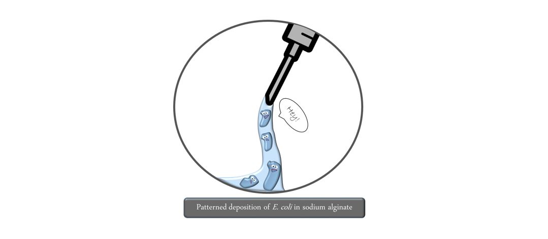
Our project is entitled Biolink and provides an alternative to current biofilm formation technologies. We use a 3D printer, which we call The Biolinker, to form layers of a designed bioink made of bacteria that can bind together into a desired structure.
Biolink helps biofilm-related industries in several ways. First, it brings reproducibility and control to how bacterial biofilms can be artificially formed. Second, biofilm printing adds automation and scalability, making biofilm formation processes more efficient, and thus, cheaper. Hence, Biolink can help to design safer and more effective anti-biofilm solutions by increasing biofilm testing process efficiency and resemblance to reality.
The Biolink Project
Our printing system, called Biolink, can be summarized in the following sentence: biofilm producing bacteria are printed with the help of a flexible scaffold hydrogel. First of all, our homemade bacteria (modified to make biofilms) are mixed with a solution of sodium alginate and subsequently with calcium chloride. There, the Ca2+ molecules keep the structure fixed creating a stable gel. This hydrogel-bacteria mixture is then induced with rhamnose, a sugar specific for our promoter, which makes them synthesize CsgA, the linking molecule. CsgA proteins polymerize to an amyloid structure surrounding the cells and connecting them to each other through the scaffold. Once the cells are all attached in the structure defined by the gel scaffold, it is no longer necessary. Consequently, the hydrogel is dissolved with sodium citrate. But the cells are still connected due to the curli amyloid! So, we obtain a perfectly defined 3D structure made of bacteria.


The Biolink project promotes the open source and educational spirit of iGEM. Our 3D printer, the Biolinker, is made of K’NEX construction toys, a DIY solution that is both easy to build and efficient in doing its job. Through policy and practice we try to position our project within the synthetic biology industry and academia, as well as observe socio-economic perception and feedback. We accomplish this by analyzing and interviewing stakeholders, treating ethical and regulatory issues, and building a business plan around our project.
Synthetic Biology in our Project
During biofilm formation, bacteria produce an extracellular matrix made of amyloid structures. These amyloid structures are curli fimbriae, composed of intertwined filaments with a thickness of approximately 4-7 nm (Nguyen, 2014). Therefore, curli production helps bacteria bind to each other in natural biofilms (Taylor et. al. 2012). There are two distinctive operons involved in this highly regulated pathway; csgBA and csgDEFG. The csgBA operon encodes for two proteins: CsgA and CsgB. The csgDEFG operon encodes for the proteins required for the transport of CsgA and CsgB to the cell surface (Dueholm et al, 2011).
On one hand, CsgA is an amyloid protein that acts as monomer for curli formation. On the other hand, the protein CsgB in an integral membrane protein, which binds CsgA to the cell; CsgB acts as an anchor for curli formation. CsgA is transported as an unfolded protein to the extracellular matrix. Once outside the cell, it aggregates with CsgB and the self-assembly of these aggregates form the amyloid fibrils. When CsgA comes in contact with CsgB, the fibrils bind to another cell and the process is repeated again until an entire network has been created (Barnhart et al, 2006).
In our project, we designed an inducible system for synthesizing CsgA in biofilm-making deficient cells. Besides to that, we aimed to create a customized biofilm. To do so, we designed different biobricks that contain a peptide tail attached to the sequence of the biofilm protein CsgA that provides a specific surface affinity. In the end, we planned to use our engineered cells (which also express a fluorescent reporter) for printing in different layers; printing biofilms in 3 dimensions.
The Bioink and Alginate as Supporting Scaffold
In initial experiments printing with bacterial cells dispersed in LB media it quickly became obvious, that a supporting scaffold would be required: due to surface interactions the liquid spread out creating a final thickness of the printed line of almost one centimeter. In tissue engineering sodium alginate is commonly used as a synthetic extracellular matrix material (Rowley et al., 1999). Inspired by this, we took a look at sodium alginate to use as a scaffold material. Sodium alginate is a carbohydrate polymer which can be fairly well dissolved in water, but in contact with calcium ions (or other divalent cations) the polymers are connected via electrostatic interactions forming a hydrogel. Made for instance from LB, this hydrogel could provide bacterial cells with everything they need for weeks and keep them alive. Furthermore, jellification is a reversible process by complexing the calcium ions with citrate and replacing it again with sodium ions (Rowley et al., 1999). Thus, we had found a substance ideally meeting our purpose of being initially liquid, capable of rapidly turning into a viscous gel and reversing this process again.
Strains
The strains used for our project are described here
Escherichia coli K-12 MG1655 PRO ΔcsgA ompR234
This strain of Escherichia coli, used in previous studies of amyloid fiber production in bacteria, is characteristic for having knocked-out the CsgA gene. However, it has all the other genes required for formation of the curli structure.
We have used this strain for our project as the main organism for the printing process. As the bacteria cannot express csgA, we transformed our strains with a plasmid containing this gene under the control of an inducible promoter. Consequently, we can modulate where and when the amyloid fiber will be formed! (Chen, A.Y., et al. 2014)

Escherichia coli Top10
This strain was used exclusively for highly efficient transformations. We used this organism for cloning experiments, plasmid isolations and other basic steps of our project.

Linking Cells
The possibility of printing bacteria in structured layers is supported by the biological property of making biofilms. In this part of the project we studied the proteins that allow cells to produce connections, and how we can modulate their production
Introduction and Motivation
Printing a biofilm requires the bacteria to produce several components that allow them to make a connection between them. Furthermore, they require to attach to the surface where they are printed on. Finally, they need to make the biofilm only when it is desired.
In order to study the connections that exist between bacteria, we focused on the bacterial amyloid curli structure. These bacterial structures contribute to biofilm performances where cells interact with other cells and even surfaces. The curli consists of proteins bound together and to the cell membrane. CsgA, the main subunit, polymerizes in the extracellular space creating an amyloid nanowire; and CsgB anchors this nanowire to the membrane, creating connections between different cells (Joshi et al., 2014).
Consequently, we designed different versions of biobricks (see Parts) coding for the CsgA gene to create a biofilm in a controlled manner from CsgA deficient cells. To prevent premature biofilm formation and clogging of our printer, we designed the expression of CsgA to be inducible by rhamnose so that the biofilm is only created after the cells are printed. This also functions as a safety feature in case of escape. The experiments (and their results) that we used to analyse the expression of CsgA and its promoter are explained in this section.
Background
In the kinetic experiment, the fluorescence signal of the proteins CsgA and CsgA-GFPmut3 (I13504) proteins expressed by our constructs was recorded in time. Besides fluorescence, we measured the OD600 of our cultures in order to normalize the fluorescence signal per cell. The main goal of this experiment was to see, if different induction levels with increasing rhamnose concentrations would lead to a higher production of CsgA. If this was true, the quantity of produced CsgA present in the medium could be controlled. This degree of control is key to achieving our main goal; making a biofilm with reproducible strength.
The obtained results can be used to calculate the promoter strength at different induction levels of rhamnose in our model. In order to use the mathematical model previously constructed in the modeling section, it has to be fitted to GFPmut3 units/cell/second. Therefore, we set up a calibration curve with exactly the same settings as the fluorescent experiment in order to correlate fluorescence signal to units of GFPmut3 per cell.
Methodology
In this experiment, the strains ∆csgA – csgA- I13504 and ∆csgA – csgA strain were both induced with rhamnose at different concentrations. The different induction levels can be found in Table 1.

All conditions (ID 1 – 6) were carried out in triplicates for accurate statistical analysis of the data. The different cultures were grown and induced in a 96-well plate. The OD600 and the fluorescence signal was recorded with a plate reader during an 18-hour period at 30°C.
Results and discussion
In Figure 5, the fluorescent signal was normalized with the number of cells and plotted as a function of time. The red bars denote the error within each ID.
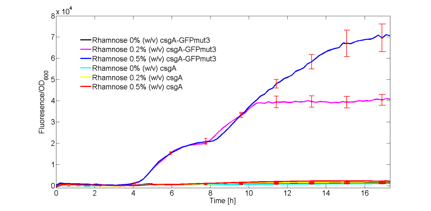
As observed in Figure 5, only the strains carrying the csgA-GFPmut3 construct induced with 0.2% (w/v) and 0.5% (w/v) showed a clear increase in fluorescence signal over time. The rest of the cultures, didn’t show significant fluorescence over time.
Furthermore, we have showed that increasing concentrations of rhamnose lead to increasing amounts of produced csgA-GFPmut3 and thus fluorescence. Finally, as the fluorescence signal is normalized by the cell density, one can make statements about the activity of the rhamnose promoter. The promoter seems to not be active directly after induction, but activity is observed after a time period of 3 to 4 hours. This is in accordance with data from literature (Wegerer et. Al, 2008), in which low fluorescence levels were observed after 2 hours of induction of the rhamnose promoter.
The calibration line of fluorescence versus mass amount GFPmut3 is given in Figure 6.

The corresponding function of the GFPmut3 calibration line is:

With massGFP in ng.
In the modelling, the fluorescent data in Figure 5 will be further converted to molecules GFPmut3/cell and the promoter activity will be calculated for both the 0.2% (w/v) and 0.5% (w/v) level of rhamnose induction. With this kinetic experiment, we have proven that our csgA-GFPmut3 construct is able to produce different levels of GFPmut3 by varying the rhamnose concentration.
Background
With our biofilm formation model we aimed to estimate how many times the nanowires overlap in order to predict the biofilm strength. One of the variables required for this model is the persistence length. In order to determine it, we have to visualize the nanowires produced by our engineered bacteria. Moreover we wanted to visualize the difference between induced and uninduced cultures containing the csgA_pSB1C3 plasmid with a rhamnose inducible promoter. These experiments required using an electron microscope.
Electron microscopes use electrons to visualize nano-objects, such as the curli nanowires. In the large “gun” the electrons get enough space to accelerate before they illuminate the sample. As shown in Figure 7 after the electrons are fired by the gun, an electric field of several thousand volts is applied to the electron beam in order to point this to the sample. In the case of an TEM, the electrons pass through the sample where the detector can detect the sample (Boysen & Muir, 2011).

Methodology
At first we measured an OD600 of 3.00 of an overnight culture of ∆csgA_csgA_pSB1C3 cells. We diluted the sample down to an OD600 of approximately 0.05, with LB medium + CAM (antibiotic, chloramphenicol). To achieve an end volume of 4 mL we took 67 µl of the overnight culture and 3933 µl of LB + CAM. We let the cells in the new sample grow for 1.5 hour at 37°C to reach the exponential phase (OD between 0.35-0.60). After the cells reached the exponential phase, we induced 1 mL of the culture with 1% rhamnose (250 µl from our 5% rhamnose stock) and also took 1 mL sample of the uninduced culture. We incubated both samples overnight at room temperature to allow the production of nanowires. Finally, the samples were directly added to the grid and the following TEM pictures were taken.
Results

In Figure 8, both the situation, pictured with TEM, without induction (the left one) and with induction (the right one) are shown with a magnification of 7300 x. The situation in which there was no induction with rhamnose, the bacteria did not show any curli formation. The opposite was true for the case in which the cells were induced with rhamnose. As the TEM picture clearly shows, nanowires are present after induction.
Background
The bacteria that we engineered for the project are capable of producing curli proteins after induction with L-rhamnose. However, the goal of our project is the printing of biofilms and not the sole overexpression of these proteins. In order to assess whether our CsgA-producing bacteria can make a biofilm or just remains planktonic, our team adapted the protocol from Zhou et al. (2013) that employs crystal violet (methyl violet 10B) for dying the biofilm-making bacteria that attach to surfaces.
According to the source article (Zhou et al., 2013), a deficient mutant of Escherichia coli is unable to produce a biofilm. By performing this experiment, we want to go further in characterizing our curli proteins; we want to answer this question: are we really making biofilms?
Methodology
In the experiment, our CsgA-producing strain of E.coli is induced at a high (0.5% w/v), low (0.2% w/v) and no (0% w/v) concentration of L-rhamnose. Furthermore, csgA deficient bacteria transformed with an empty plasmid (pSB1C3) are also tested and used as a control (Table 2.). All the experiments were carried out in triplicates.

The cultures of both strains were grown and induced in a 96-well plate. 40 hours after the induction, the samples were washed with water (in order to disregard non-attached, planktonic cells) and dyed with crystal violet (figure 9.).

Results and discussion
In the end, the wells were diluted with ethanol so all the content can dissolve in the liquid phase. We measured the absorbance at 590 nm of wavelength for all the samples, obtaining the following results (figure 10.):

The cells induced with l-rhamnose showed an increased absorbance at 590 (the peak of the dye) when compared to the empty-plasmid controls, and also with the non-induced sample. That results clearly demonstrate how our engineered cells with BBa_K1583000 successfully make biofilms, regarding that the empty plasmid controls and the analysed samples have significantly (table 3.) higher crystal violet retention. On the other hand, a higher concentration of rhamnose is not leading to a higher expression. The cells induced with a 0.2% w/v of rhamnose seem to create better a biofilm structure. However, this could be a consequence of different growth patterns; the cultures induced with 0.5% w/v of rhamnose could have stopped duplicating earlier, so the cell concentration could have decreased. So, the dyed area could be consequently smaller.

Background
For the kinetic model, we needed to determine the internal concentration of csgA. We cloned a CsgA gene, with a C-terminus His tag, in the construct in a CsgA deficient strain. The His-tag would give us the advantage to use multiple techniques, for measuring the amount of CsgA proteins. Based on the kinetic experiment with GFPmut3, we obtained an internal amount of CsgA in the order of 104 molecules/cell. To validate whether this value was plausible we decided to use a sensitive, and an accurate method: the Western Blot.
Methodology
Experiment 1: Qualitative analysis of internal CsgA_His protein
We performed the Western Blot according to protocol 24. The following samples (Table 4) were used for performing the Western Blotting experiment.

Alternative steps were done during step 5 of the protocol. After incubation we removed the medium, by centrifugation at 4000 rpm for 15 minutes at 4000 rpm. The supernatant was discarded, and the cells were resuspended in sample buffer to obtain an OD600 of 10. The cells were then heated for 10 minutes at 95°C, followed by centrifugation for 5 minutes at 32000 rpm at 4°C. This was then continued with step 6. For step 6, we added 10 µl per slot in the SDS page gel.
Experiment 2: Quantitative analysis of the internal CsgA_His protein.
We executed a second experiment to quantify the amount of CsgA_His present in the ΔcsgA_csgA strain. We compared this amount by using a the T-SSRA madrid proteïn solution. T-SSRA madrid proteïn solution has a set amount of proteins with the His tag on it. Therefore by using the Lambert-Beer law, the concentration of proteïn was calculated to be 200µM. We used a dilution series of 1/10, 1/25,1/50, 1/100, 1/500, 1/1000 (Table 5) in order to make a calibration curve.

The Western Blot protocol (nr 24) was followed, as executed in experiment 1.
Results and discussion
Experiment 1: Qualitative analysis of internal CsgA_His protein
In Figure 11A, the SDS page gel is shown. The gel is too condensed to visualize a difference between the non-induced and induced samples, because the gel was overloaded.


We saw in figure 11B a band in lane 4 and 8, with a size of circa. 17 kDA. The lanes correspond to the strain ΔcsgA_csgA_his induced rhamnose, after 5 hours and 24 hours of induction. The antibodies bind specifically to the His-tag of proteins, which did not bind to the ΔcsgA_csgA samples, line 1, 2, 5 and 6. Therefore it can be concluded that the strain ΔcsgA_csgA_his produced his-tagged CsgA proteins. The effect of rhamnose was visible when compared to the samples with ΔcsgA_csgA_his without rhamnose induction, lane 3 and 7. There are no bands visible, therefore rhamnose induces the production of CsgA_His. We can conclude with experiment 1 that the antibodies bind specifically to CsgA_His proteins. The CsgA_His proteins are only present when induced with 0.5% rhamnose.
Experiment 2: Quantitative analysis of the internal CsgA_His protein.
With experiment 1 we proved that the antibodies bind to CsgA_His proteins. The CsgA_His strains produced CsgA_His after induction with 0.5% rhamnose. We executed experiment 2 to determine the internal concentration of CsgA_His proteins, by comparing the bands with the bands of known concentrations of CsgA_His proteins.

As seen in figure 12, the bands of the calibration curve were visible. The bands of the ΔcsgA_csgA_His were not visible. We still wanted to know the correlation between the thickness of the band, and the concentration of internal CsgA_His. We solved this by comparing the band in lane 8 from figure 11B with the bands seen in figure 11A, to acquire an approximation of the total concentration. The bands in lane 4, and 5 (right to left) were too saturated to measure with the Typhoon. The band in figure 2 was thinner than the two highest concentrations, therefore we removed the last two points from the calibration line.
The trend line of the concentration (in µM) versus intensity has a formula of:
Intensity = 509067 · [concentration] + 792496
We calculated from figure 11B that the average intensity of our samples 2.3*10^6 was. We used the calibration curve (figure 13) we made with the dilution series to determine the average CsgA-His amount per well to be 2.75 μM. The amount of sample we loaded on the gel was 10 µl, therefore the amount of CsgA_His protein in the lane 2.7510-5µmol.

The cell concentration was set to an OD600 of 10 at the beginning of the experiment, which corresponds to 8109 cells/ml. 10 µl of this suspension was loaded per gel slot. With the number of cells and the amount of CsgA per slot known we were able to calculate the number of CsgA proteïns per cell: 2.06105 molecules/cell.
Conclusions and Future Directions
With the experiments described previously we achieved biofilm formation with our harmless lab Escherichia coli strains. Also, we managed to limit this expression only when rhamnose (a metabolizable inductor) is supplied. In overall, these results show a promising genetic construct to be used for bio-printing purposes. However, the experiments conducted in that part of the project could not really determine the exact effect of the induction level (i.e. concentration of rhamnose) in the biofilm formation. So, we would like to advise future researchers in this field to look for more detailed and complex experiments that could give information about the biofilm structure differences in time.
Next to the linking experiments, a step further in biofilm design would be to endow our strains with surface-attachment capability. This property will be analysed in the next part of our project, Affinity Tags.
Affinity Tags
In this section we worked in the characterization of strains that display special affinity to certain surfaces.
Introduction and Motivation
In our aim to develop a fully customizable biofilm formation process, we wanted to improve their adhesive properties and make them stick to any possible surface. To achieve this goal, we modified the CsgA protein (monomer of the curli nanowire) and added affinity tags to it. First of all, we thought about biofilms that naturally grow in our mouths. These biofilms are a major issue in testing antibacterial products like toothpastes, so we thought we could contribute to that process by adding an affinity tag for the dental surface. Moreover we also designed other affinity tags of interest. The complete list is shown in Table 6:

In the following section, we have analyzed the biofilm-making ability of the strains carrying the plasmids containing the modified csgA sequences. Also, for the HA tag (hydroxyapatite), we have designed an experiment for evaluating the attachment specificity of the modified amyloid to the dental surface.
Background
The bacteria that we engineered for the project are capable of producing curli proteins after induction with L-rhamnose. We assessed whether our CsgA-producing bacteria can make a ring-shaped biofilm by adapting the protocol from Zhou et al. (2013) using crystal violet for dying the biofilm-making bacteria. However, now we would like to know if the cells that we engineered to have a special affinity for different surfaces can also make biofilms. For that reason, we repeated the assay with crystal violet for the different strains that produce CsgA but contained in a different plasmid.
Methodology
In the experiment, our CsgA-producing strain of E. coli is induced at a high (0.5% w/v), low (0.2% w/v) and no (0% w/v) concentration of L-rhamnose. Furthermore, csgA-deficient bacteria transformed with an empty plasmid (pSB1C3) are also tested and used as a control (Table 7). All the experiments were carried out in triplicates. A summary of the samples used for the experiment is also shown in Table 7:

The cultures of all the transformed strains were grown and induced in a 96-well plate. 40 hours after the induction, the samples were washed with water (in order to disregard non-attached, planktonic cells) and dyed with crystal violet. Finally, the wells were filled with ethanol so all the content can dissolve in the liquid phase and be measured in the plate reader in triplicates.
Results and discussion
The absorbance at 590 nm of wavelength is measured for all the samples, obtaining the following results displayed as bar plots (figure 14, 15, 16, 17, and 18):


As we also observed in the crystal violet assay for the plasmid containing the csgA gene, the sample that can also express RFP as a reporter gene is also able to make a biofilm. That confirms that this strain can be used for the experiments of characterization of the 3D printing, as the reporter gene expression is not interfering in the biofilm-making ability.
On the other hand, the tagged CsgA proteins seem to have biofilm-making capability despite having a peptidic modification in the structure. To confirm that there is a real change between the analysed samples and the empty plasmid control, a significance analysis was performed for α=0.05 (Table 8.).

The significance analysis shows how all the samples with a modified CsgA can efficiently create a biofilm, when compared with an empty plasmid control (i.e. without csgA expression). The sample with CsgA and RFP as reporter gene, when induced with 0.5% w/v of rhamnose, shows no significant difference with an alpha value of 0.05. However, if we look at the p-value (0.0503) we can see that it is actually really close to a 5% of significance. So, the variation could be due to the manipulation.
We could conclude that the tags added to the CsgA molecule do not have a negative effect on biofilm formation, but also that the rhamnose concentration used for induction do not have a remarkable effect for such a long induction. Now that the biofilm capability of these strains is proved, proper function tests for the affinity tags are required. With that, we could confirm that we have generated biofilm with special affinity for certain surfaces.
Background
In our research for a highly representative biofilm that could be used for testing products, we thought about the main surfaces where a non-desirable biofilm can be attached. The first structure that came into our minds was the dental cavity; there, biofilms can attach to the tooth cover and create strong and resistant biofilms (Kidd, E.A., et al, 2004).
In our research about the dental surface we found that the external part that protects the inner tooth fragments is the enamel. Hydroxyapatite (Ca10(PO4)6(OH)2), also known as bone mineral, is a mineral compound that represents the major inorganic part of the dental enamel and dentin (Staines,M. et al, 1981). Thus, we looked forward to a way to make our biofilm attach better into a hydroxyapatite-covered surface.
In the end, we found that our homemade biofilm could be improved with surface-specificity just by adding a particular tag attached to our amyloid protein, CsgA (Roy,M. et al, 2008). This tag, successfully added to our csgA construct and cloned in our vehicle strain, does successfully make biofilms when induced with rhamnose. However, we thought that the best way to prove that it can resemble a real mouth-attached biofilm is testing it with teeth!

Methodology
For the experiment aiming to prove that our biofilm can be strongly linked to the enamel surface, we managed to get some teeth from a cow (Bos taurus) (figure 19.). We cut them in small pieces of similar size (~1cm3) and place them in a 96-well plate. Afterwards the well was filled with 5 mL of cell culture, induced and incubated for 40 hours at room temperature, without shaking. The strains used for the investigation are summarized in table 9:

Once the dental pieces had enough time to be covered with specific curli-generating cells, we designed two different protocols for measuring the efficiency of the affinity tag. In both cases, the cells were expressing RFP (red fluorescent protein) under a constitutive promoter. Thus, the number of cells that remained attached to the surface could be calculated out of the fluorescence intensity.
We tried to measure the remaining cells attached to the dental surface after submerging it in water for 2 seconds. The first approach included a direct measurement technique: measuring RFP presence using a Typhoon ® Fluorescence Scanner (figure 20).

On the other hand, we also measured the cells attached to the tooth by putting the samples in an ethanol (70%) solution for 5 minutes. Consequently, the cells will detach and float in the supernatant. When we measure the fluorescence intensity of this ethanol supernatant, we will be able to discriminate if there is actually a difference in the attachment properties of tagged and untagged cells. Detailed information of the nomenclature used in the figures of this section can be found in table 10.


Results and discussion
We tested the RFP presence in the tooth samples (figure 21) with a fluorescence scanner, obtaining the following results (figure 22):

The results of this experiment showed a strong background from the samples, meaning that probably the teeth display some kind of self-fluorescence. Consequently, the results of this test cannot be considered for proving the affinity to hydroxyapatite of our biofilms.
Then we performed the second measurement assay, using a 96-well plate and the plate reader. The results are displayed in figure 23, and the parameters were confirmed using the supernatant of the CsgA producing cells with no ethanol treatment.

From the results shown above, we could conclude that our affinity tag for hydroxyapatite gives an actual difference when compared with the control samples, for significance level of 5%. Also, the statistical analysis confirms that there is a significant change between cells with the affinity tag and without it (Table 11).

Our initial plan was to, in addition to the His- and Hydroxyapatite-tag, also attach a SpyTag to the CsgA proteins. This idea was based on an article of the Joshi Lab on programmable biofilm-based materials (Nguyen, Botyanszki, Tay, & Joshi, 2014). This SpyTag can spontaneously form covalent bonds with a protein called SpyCatcher. The SpyCatcher protein can be attached to other proteins to form a fusion protein. This way the fusion protein can be immobilized on the SpyTag. By attaching the SpyTag to the CsgA protein, the SpyCatcher can indirectly bind to the nanowires formed by CsgA. This way fusion proteins can be immobilized on the nanowires and a functionalized biofilm can be created. (Nguyen et al., 2014)
To prove that this mechanism works, we envisioned to make a fusion protein of SpyCatcher and amylase, a protein that catalyses the hydrolysis of starch. Amylase is actively transported out of the cell and thereby a biofilm could be created that produces both the nanowires and the enzymes that will be immobilized on these nanowires. However, shortly after coming up with this idea, a paper was published on exactly this system. (Botyanszki, Tay, Nguyen, Nussbaumer, & Joshi, 2015). This showed us that using the SpyTag/SpyCatcher system to immobilize enzymes on the nanowires was indeed deemed interesting.
To at least prove that this idea could work with our biobricks, we created a fusion protein of Blue Fluorescent Protein (BFP) with SpyCatcher (BBa_K1583113). The BFP could be easily assessed on its fluorescent properties to see whether it could still properly function and fold when attached to SpyCatcher. However, we experienced difficulties with the construction of both the CsgA_SpyTag biobrick and the BFP_SpyCatcher_His biobricks. Unfortunately CsgA_SpyTag contained a frameshift, that proved to be hard to remove and the arabinose induction of BFP_SpyCatcher_His also did not work as expected. Still, since we do very much like the idea of creating functionalized biofilms in this manner, we still wanted to explain this idea here and hope that future iGEM teams can successfully conduct this experiment.
Conclusions and Future Directions
These experiments represent a big step in biofilm customization, allowing researchers to create biofilm structures that bind specifically to certain surfaces. Nevertheless, this could be only used as an extra for 3D biofilm printing, as linking cells between them seems to be the limiting step for printing with our hardware prototype.
We have tested that the strains producing CsgA with the different affinity tags can still form biofilms despite having a peptidic modification in the CsgA structure. However, the affinity test has been performed for the hydroxyapatite (HA) tag and the polyhistidine (His) tag, meaning that the binding capabilities of the mfp3 and mfp5 tags still have to be proven.
Our initial plan was to, in addition to the His- and Hydroxyapatite-tag, also attach a SpyTag to the CsgA protein. This idea was based on an article of the Joshi Lab on programmable biofilm-based materials (Nguyen, Botyanszki, Tay, & Joshi, 2014). The SpyTag can spontaneously form a covalent isopeptide bond with a protein called SpyCatcher. The SpyCatcher protein can be attached to other proteins to form a fusion protein. This way the fusion protein can be immobilized on the nanowire by means of the SpyTag. By attaching the SpyTag to the CsgA protein, the SpyCatcher can indirectly bind to the nanowires formed by the CsgA. This way fusion proteins can be immobilized on the nanowires and a functionalized biofilm can be created.(Nguyen et al., 2014)
Printing Biofilm Layers Using Fluorescent Cells
Our final goal in the project was the ordered printing of biofilm layers. So, in the following part we describe how we did that and how we achieved 3D printing of biofilms
Introduction
One of the goals of our project is to print biofilms with a defined structure. This could be applied in e.g. industrial processes in which the production pathway is divided over several organisms (Zhou et al. 2015). An example of such a process is given below (Figure 24). The orange substrate is converted by the blue bacterium to the purple intermediate. This purple intermediate is converted by the red bacterium to the green final product. This conversion can be done in two separate reactors, in which case purification steps are required in between the two reactors.
Another option is to do the conversion in one reaction. In this case the outflow will contain not only the end product, but also substrate and intermediates. When you would be able to optimally structure the two bacteria, the produced intermediates would be directly converted by the red bacteria, thereby minimizing the amount of intermediates in your outflow and thereby increasing your yield.
Also in the case that the purple intermediates inhibit their own production (feedback inhibition), structuring the bacteria and thereby minimizing the intermediate concentration could have a beneficial effect on the yield (Kiely, Regan, and Logan 2011).

To be able to make structured biofilms of different (types) of bacteria, it is important that we prove that we are able to structure the bacteria and that these bacteria stay in place.
To prove this we used cells producing the fluorescent proteins GFP and RFP, to resemble different strains in an industrial process. To to show that we can structure these cells and that they do not mix, we wanted to assess the distribution of the cells after printing with confocal microscopy (Figure 2).

We have transformed TOP10 cells with the plasmids I27020 (GFP) and I13521 (RFP) (Table 12.). We grew cultures of these cells overnight in 5 mL LB with antibiotics. To obtain 500 μL of bio-ink, 1 mL of cells was spun down at 4000 rpm for 3 minutes and the supernatant discarded. We added 100 μL of sterile LB, resuspended the cells and then added 400 μL of 1% w/v sodium alginate. This mixture was vortexed to ensure that the cells are homogeneously distributed. The formation of the hydrogel by alginate and CaCl2 is discussed in more detail in the hardware section.

To be able to visualize the cells, the bio-ink needed to be printed on a coverslip suitable for the spinning disk microscope instead of the usual agar plates (See hardware). We used plasma-cleaned coverslips, since the normal coverslips are very hydrophobic and cause liquids to form a bubble on top of the surface. Plasma cleaning removes the impurities and contaminants on the coverslip and negatively charges the surface, thereby rendering it hydrophilic. This way contact between the coverslip and the bio-ink is improved.
For printing the layers of bio-ink, we first made a line of the alginate with RFP cells on the coverslip (Figure 3). This was done in the first experiment (Layer formation) by extruding the bio-ink at a flow rate of 100 uL/min with the syringe pump. In the second experiment (3D-stack), we used a 1-10 μL pipet. After printing of the first layer, CaCl2 was added on top of the alginate to start the formation of the hydrogel. We discarded the excess of CaCl2 by tilting the coverslip and removing the liquid with a tissue. This makes the layers of alginate a bit thinner, which is beneficial for the image quality with the spinning disk microscope. The image quality improves because the shorter distance to the objective leads to a lower background signal. The layers on top of this first layer we applied in the same manner.

Normally, the bio-ink is printed on an agar plate containing CaCl2. When the bio-ink gets into contact with the agar, the CaCl2 reacts with the alginate to form the hydrogel. To be able to better represent the printing with the DIY printer, we also tried to first apply a layer of CaCl2 on the coverslip and print the layers of bio-ink on top of this. However, the results was that the alginate would float around in the CaCl2, and it was not possible to make several layers of bio-ink on top of each other in a structured way.
Layer formation
We used the syringe pump to make four layers of the bio-ink, with cells containing RFP on the bottom and layers of cells containing GFP, RFP and GFP, respectively, on top of that. This sample was imaged with a spinning disk microscope at 488 nm and 561 nm, for the excitation of respectively GFP and RFP (Figure 27).

As can be seen in figure 27, the first layer does contain red cells (1.2), but does not contain green cells (1.1). The same holds for layer three (3.1 & 3.2). Layer two and four both contain green cells (2.1 & 4.1), while they both do not contain red cells (2.2 & 4.2). The visibility of the cells in layer three and four is reduced due to their increased distance from objective, which results in a higher background signal. This spatial distribution of the cells proves that we can make distinct layers of cells.
3D-stack
We proved that we are able to make distinct layers of cells, but we did not know yet whether there was a mixture of the different cells at the interface between two layers, or whether they are clearly separated. Also we did not know yet how thick the layers were. To test this, we made a new sample with two layers and took images with the spinning disk microscope in 74 planes over a distance of 146 μm at the same two wavelengths. Of these planes, 34 were used to make a 3D stack of the sample (Figure 28ab). As a control to show that the hydrogel formation assists in layer formation, layers of red and green cells were printed without alginate and CaCl2. Images of 76 planes over a distance of 37.5 μm with excitation at 488 nm and 561 nm were taken and of these 36 were used to make a 3D stack (Figure 28cd).

This image shows that two distinct layers are formed when bio-ink was used and mixing between the layers is almost negligible. The height of the red layer is around 29 μm and the height of the green layer is around 34 μm depending on the position in the layer. The sample without alginate shows that without the use of bio-ink, the cells are not structured and a mixture of red and green cells is formed. This proves that the hydrogel assists in layer formation and that we can use this system for printing the biofilm; the cells can be printed in a structured way and no mixing occurs, even at the interfaces between layers.
Conclusions and Future Directions
We started these experiments with the question whether we can print biofilms in a defined structure. To assess whether we can do this, we wanted to show that we can structure the cells and that they do not mix. The first experiment, layer formation, showed that we can indeed structure the cells in layers. In the second experiment, 3D-stack, we additionally proved that these layers are separated from each other and do not mix. Therefore we conclude that we can print bacteria in a defined structure.
The iGEM team Groningen already set the foundation to the future, where our developed procedure could be tested on different species of bacteria, to assess whether they can also be printed in layers. Supported by interest from industry, further experiments with an applied focus could prove very interesting.
References
Kiely, Patrick D, John M Regan, and Bruce E Logan. 2011. “The Electric Picnic: Synergistic Requirements for Exoelectrogenic Microbial Communities.” Current opinion in biotechnology 22(3): 378–85. http://www.ncbi.nlm.nih.gov/pubmed/21441020 (September 17, 2015).
Zhou, Kang, Kangjian Qiao, Steven Edgar, and Gregory Stephanopoulos. 2015. “Distributing a Metabolic Pathway among a Microbial Consortium Enhances Production of Natural Products.” Nature Biotechnology 33(4): 377–83. http://www.nature.com/doifinder/10.1038/nbt.3095 (January 5, 2015).
Kidd, E. A. M., & Fejerskov, O. (2004). What constitutes dental caries? Histopathology of carious enamel and dentin related to the action of cariogenic biofilms. Journal of dental research, 83(suppl 1), C35-C38.
M. Staines, W. H. Robinson and J. A. A. Hood (1981). "Spherical indentation of tooth enamel". Journal of Materials Science 16 (9): 2551–2556.
Roy, M. D., Stanley, S. K., Amis, E. J., & Becker, M. L. (2008). Identification of a Highly Specific Hydroxyapatite‐binding Peptide using Phage Display. Advanced Materials, 20(10), 1830-1836.
Zhong, C., Gurry, T., Cheng, A. A., Downey, J., Deng, Z., Stultz, C. M., & Lu, T. K. (2014). Strong underwater adhesives made by self-assembling multi-protein nanofibres. Nature nanotechnology.
Chen, A. Y., Deng, Z., Billings, A. N., Seker, U. O., Lu, M. Y., Citorik, R. J., ... & Lu, T. K. (2014). Synthesis and patterning of tunable multiscale materials with engineered cells. Nature materials, 13(5), 515-523.
Barnhart, M. M., & Chapman, M. R. (2006). Curli biogenesis and function. Annual review of microbiology, 60, 131.
Wegerer, A., Sun, T., & Altenbuchner, J. (2008). Optimization of an E. coli L-rhamnose-inducible expression vector: test of various genetic module combinations. BMC biotechnology, 8(1), 2.
Earl Boysen and Nancy C. Muir (2015) See at the Nano Level with Electron Microscopy, Available at: http://www.dummies.com/how-to/content/see-at-the-nano-level-with-electron-microscopy.html (Accessed: September 2015).
Rowley, J. A., Madlambayan, G., & Mooney, D. J. (1999). Alginate hydrogels as synthetic extracellular matrix materials. Biomaterials, 20(1), 45-53.
Nguyen, P.Q., Botyanszki, Z., Tay, P.K., Joshi, N.S.. (2014). Programmable biofilm-based materials from engineered curli nanofibres. Nat Commun, 17(5), 4945.
Taylor JD, Zhou Y, Salgado PS, Patwardhan A, McGuffie M, Pape T, Grabe G, Ashman E, Constable SC, Simpson PJ, Lee WC, Cota E, Chapman MR, Matthews SJ. (2011). Atomic resolution insights into curli fiber biogenesis. Structure. 19(9):1307-16.
Dueholm MS1, Nielsen SB, Hein KL, Nissen P, Chapman M, Christiansen G, Nielsen PH, Otzen DE. (2011). Fibrillation of the major curli subunit CsgA under a wide range of conditions implies a robust design of aggregation. Biochemistry. 4;50(39):8281-90.