Difference between revisions of "Team:EPF Lausanne/Modeling"
| Line 846: | Line 846: | ||
\frac{\alpha_i}{\alpha_b} \approx 0.6 | \frac{\alpha_i}{\alpha_b} \approx 0.6 | ||
\] | \] | ||
| + | However, in our model of dCas9-gRNA binding, we used \(\alpha_i\approx 0\). This simplification is justified by the fact that the inhibited level is very closed to the autofluorscence. Thus taking into account the leakiness of inhibition will take the model closer to reality, but it will also be more complex and less informative. Here, the goal of the modeling is not to reproduce exactly experimental results or fit unknown parameter but its rather to have a computational tool which describe qualitatively well our bio-transistors and which can be used to design complex logic circuits. Therefore, neglecting \(\alpha_i\) (which does not appears anywhere on the inhibition kinetic model), we have the following response of our transistor.</p> | ||
| + | |||
| + | <center> | ||
| + | </br> | ||
| + | <figure> | ||
| + | <img src="https://static.igem.org/mediawiki/2015/e/ef/Inhibition_E._coli.png" style="height:48%;width:48%;" /> | ||
| + | <figcaption>Activated GFP expression in E. coli.</figcaption> | ||
| + | </figure> | ||
| + | </br> | ||
| + | </center> | ||
</div> | </div> | ||
</div> | </div> | ||
Revision as of 18:21, 17 September 2015
Introduction
In our project, multiple transistor elements are assembled to create logic gates. We envision the chaining of such gates in order to create complex logic circuits within cells. Predicting the behavior of these complex cascades of reactions and way they reach a stationary state can be challenging. Modeling here represents the best way to understand our system and quantify the influence of various biochemical parameters. On the long run, modeling may also help fine-tune the design of biological systems and wet lab experiments.
Since the wet lab is normally accessible only during the summer, the time available for experiments during the iGEM competition is very limited. Our team were able to build a solid proof of concept of a new way of building logic circuits using dCas9, but creating a whole complex circuit would require more time. However, a good model (tuned on the experiment we performed for single transistors) allows the design and the study of complex circuits in silico.
We attempted to model the dynamics of our system's components to predict the temporal response of our biological circuits. In order to achieve a good description we initially used the powerful tools of statistical mechanics in order to generalize Hill's description of ligand-receptor binding [1] taking into account a possible interaction between two dCas9 binding to the same promoter. This statistical view of regulatory dynamic is then used, following the same steps of the simple ligand-receptor binding, to write kinetic equations.
Kinetic equations forms a system of ODEs which is solved numerically and fitted to some experimental data, in order to describe the actual dynamic of the system. We found that our model considered at the steady state is able to satisfactory describe experimental results and can be used to predict the output of complex logic circuits.
dCas9 binding models
In the following text we will often call dCas9 our dCas9 protein fused with the RNA polymerase recruiting unit. This unit is called \(omega\) in E. coli and VP64 in S. cerevisiae.
dCas9-\(\omega\) and dCas9-VP64 structures
It is often important to visualize proteins, as their 3-D structure can give information about functionality. Unfortunately, a PDB (Protein Data Bank, [17]) file for dCas9-\(\omega\) or dCas9-VP64 is not available as X-ray crystallography data on this protein are lacking. However, it is possible to extract the \(\omega\) subunit directly from the RNA polymerase (RNAP) and align it with the dCas9 protein structure.
We will focus here on dCas9-\(\omega\), as for dCas9-VP64 the same conclusions hold. All manipulations are performed with the VMD (Visual Molecular Dynamics, [18]) software and final images are rendered with Pixar's RenderMan rendering engine. We extracted the \(\omega\) subunit from the E. coli RNA polymerase (PDB 3LU0, [19]). This subunit is then aligned to the dCas9 protein (PDB 4ZT9, [20]) in order to keep the continuity on the DNA sequence. This means that the subunit is placed at the right place with respect do dCas9, but its orientation may be wrong.
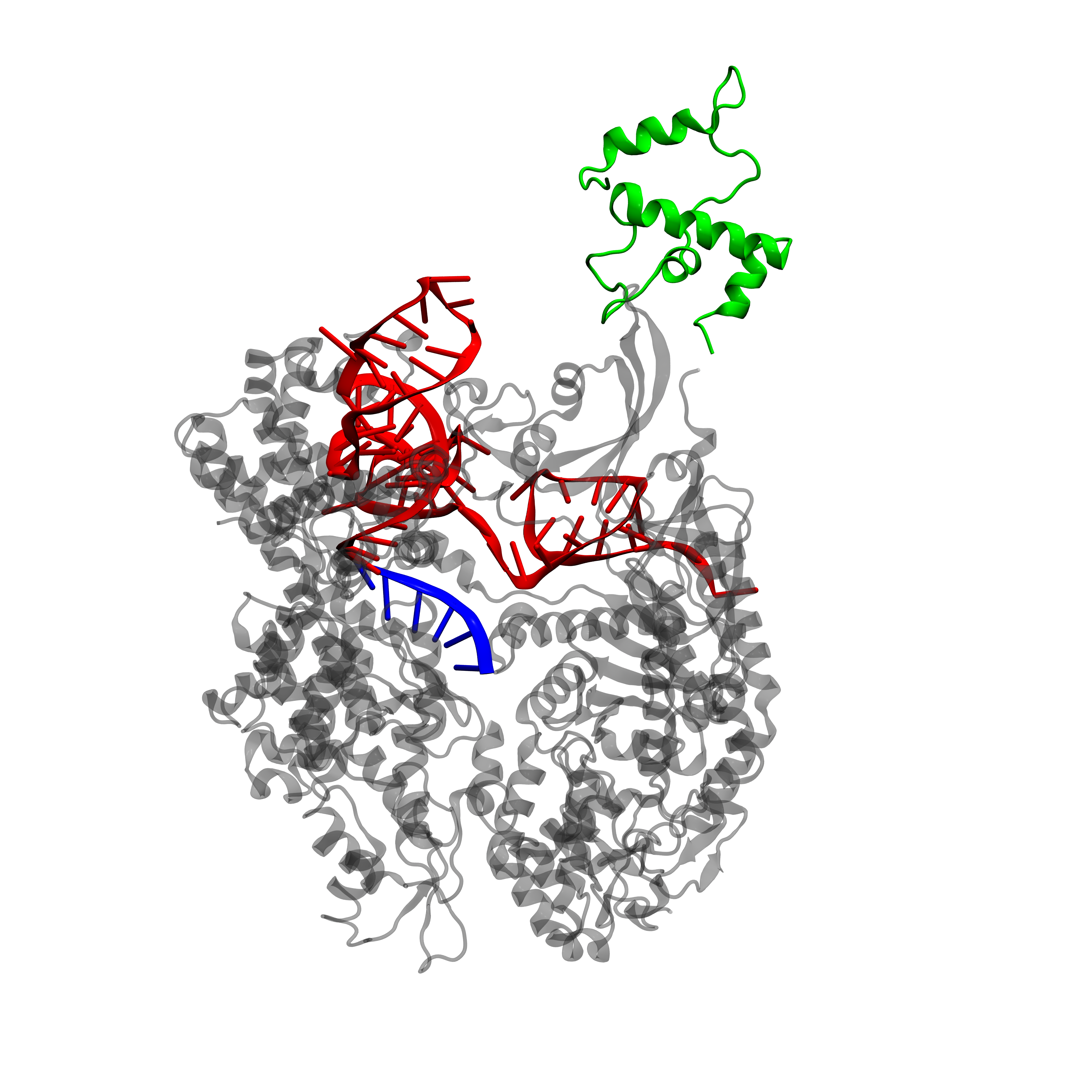
From the protein structure we can estimate the size of dCas9 on the DNA: the length along the direction of the DNA binding site is approximately 80 Å. In E. coli the distance between the activating and inhibiting sequences is of 33bp or 37bp (remember, we have two possible inhibiting sites), while in S. cerevisiae this distance is of 67bp. Now the length of double stranded DNA is of 3.1 Å per base [22], therefore the distance between the activating and inhibiting sites in E. coli spans from 102 Å to 115 Å while in S. cerevisiae it is 208 Å.
As activating and inhibiting sites are 20bp long (62 Å), we see that in E. coli the dCas9-gRNA targeting of one site is not necessarily independent of the state of the other site (occupied or free) while in S. cerevisiae it can be considered as such.
Statistical derivation of the Hill's function
In this section we will derive the Hill's function from statistical mechanics calculations of ligand-receptor binding. The following discussion is strongly based on Ref. [1].
In biology we are often confronted with systems containing large number of interacting particles (small molecules, proteins, DNA and RNA fragments, ...). It is often impossible to describe the system by describing each particle individually but this is not a major problem if we are interested in the average behavior of the system; the mathematical tool which allows such description is statistical mechanics. Statistical mechanics rely on the concept of microstate which is one particular realization of the microscopic arrangement of the constituents for the problem of interest [1].
In order to simplify we will consider a lattice model for particles in solution, i.e. we imagine the solution as a series of tiny boxes amongst which we can distribute the ligands [1]. To model a ligand-receptor binding, where there is one receptor and \(L\) ligands. The number of microstates \(W\) for this system is given by the number of ways \(W_f\) of arranging the \(L\) ligands inside the lattice with a free receptor plus the number of ways \(W_o\) of arranging the \(L-1\) ligands inside the lattice with an occupied receptor: \[ W = W_f + W_o = \frac{\Omega!}{L!(\Omega-L)!} + \frac{\Omega!}{(L-1)!(\Omega-L+1)!}, \] where \(\Omega\) is the total number of available lattice sites.
Each microstate has a weight, which is given by the Boltzmann factor (if you are not at ease with the concepts of statistical mechanics, we encourage you to consult Ref. [1] for a very clear and biology-friendly introduction to the subject). We suppose that the energy of one ligand in the solution is \(\epsilon_\text{sol}\) while the energy of a ligand bound to the receptor is \(\epsilon_\text{b}\). We con now write the partition function, which is \[ Z = W_f e^{-\beta L\epsilon_\text{sol}} + W_o e^{-\beta [(L-1)\epsilon_\text{sol} + \epsilon_{b}]} = \frac{\Omega!}{L!(\Omega-L)!}e^{-\beta L\epsilon_\text{sol}} + \frac{\Omega!}{(L-1)!(\Omega-L+1)!} e^{-\beta [(L-1)\epsilon_\text{sol} + \epsilon_\text{b}]}. \] The probability to have a ligand bound to the receptor is finally \[ p_\text{bound} = \dfrac{\frac{\Omega!}{(L-1)!(\Omega-L+1)!} e^{-\beta [(L-1)\epsilon_\text{sol} + \epsilon_\text{b}]}}{Z} \] This result can be simplified by the assumption that \(L\ll\Omega\), which implies [1] \[ \frac{\Omega!}{(\Omega-L)!} \approx \Omega^L. \] This gives finally, with some rearrangement \[ p_\text{bound} = \dfrac{\frac{L}{\Omega}e^{-\beta\Delta \epsilon}}{1 + \frac{L}{\Omega}e^{-\beta\Delta \epsilon}}, \] where \(\Delta \epsilon = \epsilon_\text{b}- \epsilon_\text{sol}\).
We were able to find the binding probability of one ligand to a receptor using the tools of statistical physics, but this seems unrelated to the well-known Hill's function. In order to obtain the Hill's function we can write the ligand concentration as \[ c = \frac{L}{\Omega V_0}, \] where \(V_0\) is the volume of one lattice box. We also introduce a reference concentration \(c_0=1/V_0\). Thus we can write the binding probability as \[ p_\text{bound} = \dfrac{\frac{c}{c_0}e^{-\beta\Delta \epsilon}}{1 + \frac{c}{c_0}e^{-\beta\Delta \epsilon}} \] Finally, by defining the association constant \[ K_a = \frac{1}{c_0}e^{-\beta\Delta \epsilon} \] we obtain the Hill's function of order 1, i.e. \[ H(c) = \frac{K_ac}{1+K_ac} = \frac{c}{K_d + c}, \] where \[K_d = 1/K_a\] is the dissociation constant. From this derivation it is clear that the Hill's function \(H(c)\) can be interpreted as the binding probability of ligands with a concentration \(c\).

Binding probability and interactions
Hill's function gives a ligand/receptor binding probability and will be used to model the mRNA or gRNA transcription caused by the dCas9-gRNA in the case of simple activation or inhibition. In the complex case where activation and inhibition compete we have to take into account a possible interaction between the two dCas9-gRNA complex: the presence of one complex on the activating/inhibiting sites can partially prevent the attachment of another complex. This is in particular important in E. Coli, where the distance is between 33 and 37 bp (in S. s. cerevisiae this distance is as long as 67 bp, for the best activating/inhibiting sites). The partition function of such system, following what we did in the previous section (the same lattice model and microstate counting can be applied and we took the energy of the system with a free promoter as reference), is given by \[ Z = 1 + K_a[\text{dCas9-gRNA}_a] + K_a[\text{dCas9-gRNA}_i] + K_a^2[\text{dCas9-gRNA}_a][\text{dCas9-gRNA}_i]e^{-\beta J} \] where we assumed that the association constant is the same of the activating and inhibiting dCas9-gRNA complexes (i.e. the energy of dCas9-gRNA bound to activating or inhibiting sites is the same) and where \(J\) is the interaction energy between the two complexes.
If we consider and independent binding, i.e. the complex on the activating and inhibiting sites does not interact \(J=0\), the partition function can be factorized: \[ Z_0 = \lim_{J\to 0}Z = (1+ K_a[\text{dCas9-gRNA}_a])(1+ K_a[\text{dCas9-gRNA}_i]). \] From the partition function we can easily obtain the binding probability of activating and inhibiting complexes: \[ p_a = \frac{K_a[\text{dCas9-gRNA}_a]}{Z_0} = \frac{H([\text{dCas9-gRNA}_a])}{1+K_a[\text{dCas9-gRNA}_i]} \] and \[ p_i = \frac{K_a[\text{dCas9-gRNA}_i]}{Z_0} = \frac{H([\text{dCas9-gRNA}_i])}{1+K_a[\text{dCas9-gRNA}_a]} \] as well as the probability that nothing is bound to our promoter \[ p_b = \frac{1}{Z_0}. \] where \(H\) is the standard Hill's function. The hypothesis of independence for the activating and inhibiting site obviously leads to \[ p_{ai} = \frac{K_a^2[\text{dCas9-gRNA}_a][\text{dCas9-gRNA}_b]}{Z_0} = H([\text{dCas9-gRNA}_a])H([\text{dCas9-gRNA}_b]) \] where \(H\) is always the standard hill's function. This probability is plotted as a contour plot in the following figure for clarity.

These considerations allow us to compute the response of an activated/inhibited transistor, for which we will have (using the fact that \(p_b = 1 -p_a - p_i + p_{ai} \), denoting \([A]=[\text{dCas9-gRNA}_a]\) and \([I] =[\text{dCas9-gRNA}_i] \) and setting the inhibited expression level \(\alpha_i\) to zero) \[ \alpha_\text{max}p_a + \alpha_\text{b}p_b + \alpha_{ai}p_{ai} =\alpha_b + (\alpha_\text{max}-\alpha_b) \frac{H([A])}{1+K_a[I]} - \alpha_b \frac{H([I])}{1+K_a[A]}+(\alpha_{ai}-\alpha{b})H([A])H([I]) \] Again, we can visualize the response of the system to different levels of concentrations of the activating (A) and inhibiting (I) complexes: the response is in this case the production of new gRNAs or mRNA for reporter proteins (output signals).

If we consider a completely exclusive binding (i.e. either the activator or the inhibitor complex is attached to the promoter), in our model we have to set \(J\to\infty\) (i.e. the interaction energy between two complexes goes to infinity). In this case the last term of \(Z\) wanishes and the partition function of our system is simply \[ Z_{\infty} = \lim_{J\to\infty} Z = 1 + K_a[\text{dCas9-gRNA}_a] + K_a[\text{dCas9-gRNA}_i]. \] Again, it is easy to compute binding probabilities. We have \[ p_a = \frac{K_a[\text{dCas9-gRNA}_a]}{Z_{\infty}} = \frac{K_a[\text{dCas9-gRNA}_a]}{1 + K_a[\text{dCas9-gRNA}_a] + K_a[\text{dCas9-gRNA}_i]} \] and \[ p_i = \frac{K_a[\text{dCas9-gRNA}_a]}{Z_{\infty}} = \frac{K_a[\text{dCas9-gRNA}_a]}{1 + K_a[\text{dCas9-gRNA}_a] + K_a[\text{dCas9-gRNA}_i]} \] This gives us the response of activation and inhibition when the binding is exclusive (\(p_{ai} = 0\) and again \(\alpha_i=0\)): \[ \alpha_{max}p_a + \alpha_bp_b = \alpha_maxp_a + \alpha_b(1-p_a-p_i) = (\alpha_max-\alpha_b)p_a + \alpha_b (1-p_i). \]

In the case where the interaction between the two dCas9-gRNA complexes is not negligible (because the activating/inhibiting binding sites are too close or because the persistence length of the double stranded DNA changes significantly when it is open by dCas9) we have \(J\neq 0\). The situation is more complicated but we can still computing the binding probabilities using the total partition function \(Z\). However, in this case we will have an additional non-trivial parameter to estimate which is the interaction energy \(J\).
Assumptions
Modelers of biophysical systems often have a difficult mission. They must strike a compromise between developing a very detailed and accurate model and producing a simplistic one that may be easily analyzed and compared to experimental data.
Developing models implies making a certain number of simplifications and assumptions to enable it to conform to reality. In this section we will keep track of the assumptions we made in order to clarify our model. Since the same system may be modeled using different approaches, we will justify our choices and set of assumptions.
The most important assumption underlying our kinetic model is the fact that the concentration of a given species does not depends on spatial coordinates, i.e. it is the same in every region of the cell. This assumption is quite bold but is a common approach in the literature and usually produces accurate results [1]. The validity of this assumption is limited, for some species, by the small number of molecules present in the cell and by their localization in membranes or particular organels. In some cases it may also be necessary to consider the stochastic behavior of individual trajectories rather than global averages [1].
One of the challenges we faced while building the model was the lack of readily available kinetic constants. Since dCas9 is a newly discovered gene regulation technology [2], dCas9-gRNA and dCas9-gRNA/DNA binding/unbinding kinetics are still under investigation. One may imagine that the binding/unbinding constants are somewhat related to the gRNA sequence given the different chemical properties of nucleotide sequences. However, we will consider binding/unbinding constants to be gRNA-independent. For the gRNA/dCas9 interaction, this assumption is justified by the fact that the gRNA scaffold is always the same. For the dCas9-gRNA/DNA interaction, we can justify this hypothesis by thinking of an average nucleotide composition, as our synthetic sequences are randomly generated
dCas9 degradation is a fundamental process in our system. Since high levels of dCas9 are toxic for the cell [3], a constantly varying dCas9 population is required for a signal to propagate from one gate to another (remember, the output of a gate is a gRNA which will bind to a free dCas9 in order to propagate the signal to the next gate). We can imagine two different types of degradation for the dCas9-gRNA complex : degradation of the whole complex and degradation of the gRNA's targeting sequence (resulting in a non-functional but occupied dCas9). We will neglect the last possibility since information about such mechanism are laking and because RNA bound to dCas9 is quite stable. In addition, we assumed that this degradation rate of the whole complex is the same of gRNA-free dCas9.
dCas9 and GFP degradation are slow. For these proteins we will take into account only the dilution, i.e. the concentration diminution caused by cell division.
In our project, the dCas9-gRNA complex is used as a transcription factor. It may alternatively activate or inhibit a targeted promoter. Activation and inhibition processes are modeled using fist-order Hill functions: the Hill function is interpreted as the probability of our dCas9-gRNA complex being bound to the promoter [1]. In order to use this approach, we assume implicitly that the number of dCas9-gRNA binding sites is much smaller than the number of dCas9-gRNA present in our system. In addition, since the binding dynamics of two dCas9 to adjacent binding sites on the same promoter is not know, we developed a generalized version of Hill's model in order to include dCas9/dCas9 interaction; we will consider only the two extrema of this model which are zero or infinite interaction strength.
Summary
Constants
Constats summary
The following table summarize the constants used in our model (see Equations). A detailed explanation of the estimation performed, or computations starting from the literature can be found below.
| Name | Description | Value | Source |
|---|---|---|---|
| \(\alpha_{dCas9}\) (E. coli) | mRNA encoding dCas9 production | 83 (nM/min) | Estimated |
| \(\alpha_{gRNA}\) (E. coli) | gRNA production | 498 (nM/min) | Estimated |
| \(\alpha_{GFP,b}\) (E. coli) | mRNA encoding GFP production | 83 (nM/min) | Estimated |
| \(\alpha_{dCas9}\) (S. cerevisiae) | mRNA encoding dCas9 production | ||
| \(\alpha_{gRNA}\) (S. cerevisiae) | gRNA production | ||
| \(\alpha_{GFP}\) (S. cerevisiae) | mRNA encoding GFP production | ||
| \(\beta_{dCas9}\) (E. coli) | dCas9 production from mRNA | 2 (1/min) | CyberCell Database |
| \(\beta_{dCas9}\) (S. cerevisiae) | dCas9 production from mRNA | ||
| \(\beta_{GFP}\) (E. coli) | GFP production from mRNA | 2 (1/min) | CyberCell Database |
| \(\beta_{GFP}\) (S. cerevisiae) | GFP production from mRNA | ||
| \(\gamma_{mRNA}\) (E. coli) | mRNA degradation | 0.2 (1/min) | Bernstein et al. [5] |
| \(\gamma_{mRNA}\) (S. cerevisiae) | mRNA degradation | 0.03 (1/min) | Wang et al. [6] |
| \(\gamma_{GFP}\) (E. coli) | GFP degradation rate | 0.03 (1/h) | BioNumber 105191 |
| \(\gamma\) (E. coli) | Dilution rate | 0.02 (1/min) | Kumar and Libchaber [14] |
| \(\gamma\) (S. cerevisiae) | Dilution rate | 0.69 (1/h) | BioNumber 108255 |
| \(K_{dCas9}\) | dCas9 and gRNA dissociation constant | 10 (nM) | Wright et al. [11] |
| \(K_{DNA}\) | dCas9/gRNA and dsDNA dissociation constant | 0.04 (nM) | O'Connell et al. [10] |
mRNA and gRNA production/degradation rates
For mRNA degradation we considered the mean half-life of Refs. [5-6] and subsequently computed the degradation rate. In Ref. [6] the mean half-life is explicitly stated, while we computed ourself the mean half-life of Ref. [5] from different E. Coli strains (since our strain is not present). Note that for an exponential decay, the half-life \(t_{1/2}\) is linked to the lifetime \(\tau\) by \[ t_{1/2} = \tau \log(2) \] and the lifetime \(\tau\) is in turn linked to the decay constant \(\Gamma\) by \[ \Gamma = \frac{1}{\tau}. \]
For gRNAs we use the same degradation rate of mRNAs.
The estimation of mRNA/gRNA production rates is more complicated as it depends on promotor characteristics. Here we assume for simplicity that all promotors are of the same kind, the only difference being the number of copies of the plasmid they are in (low-copy, medium-copy, and high-copy). We assume that within a single cell we have 5, 30 and 300 copies of low-, midium- and high-copy plasmids respectively. In E. coli we consider a weak promoter starting a transcription every 35 seconds and a strong promoter starting a transcription every 6 seconds. This means that the production rate is of 10 mRNA per minute. Now, if we suppose that the cell volume for E. coli is approximately 1µm3 and in S. cerevisiae is 60µm3 [1] we can compute the production rate of mRNAs within the whole cell. We have that GFP and dCas9 are encoded in a low-copy plasmid, while mRNAs are encoded in a medium-copy plasmid.
dCas9 and GFP production/degradation rates
For E. Coli, we found a polypeptide chain elongation rate of 12-21 amino acids per second (BioNumber 100059, [8]). Since the DNA coding for dCas9 fused with the \(\omega\) subunit is 4374bp (see BioBrick BBa_K1723000), the total number of amino acids composing the protein is 1458. This gives finally a production rate of 0.49-0.86 protein transcript per minute.
In S. cerevisiae, the polypeptide chain elongation rate is estimated to be 5.5-9.3 amino acids per second [9]. Since the DNA coding for dCas9 fused with the VP64 subunit is 4323bp (see BioBrick BBa_K1723021), we find an production rate of 0.23-0.39 protein transcript per minute.
However, the chain elongation gives only an initial lag and thus it will be neglected in our model; what is important is the rate of transcription initiation, which can be found in Ref. [12] for E. coli and in Ref. [] for S. cerevisiae.
In order to find GFP production rates, we follow exactly the same procedure we used for dCas9. The GFP used in E. coli is 717bp, while the GFP used in S. cerevisiae is 714bp.
For GFP degradation we consider the GFP(mut3) half-life time (BioNumber 105191) and we computed the degradation rate in the same way we did for mRNAs. Since GFP degradation rate is slow, it will be neglected and we will consider only the dilution rate. Dilution is estimated from the half-life of our organism. For E. coli we have a division every 40 min [14], while for S. cerevisiae we have a division every 1-2 hours (BioNumber 108255).
Fod dCas9 we weren't able to find a satisfactory degradation rate. However, it turns out that dCas9 degrade slowly [13] and again we decided to neglect this degradation compared to dilution.
Equations
In the following text we will call, for simplicity, dCas9 our dCas9 protein fused with the RNA polymerase recruiting unit. This unit is called \(\omega\) in E. coli and VP64 in S. cerevisiae.
Activation
Our activation model consists of a simple transistor that takes a dCas9-gRNA complex as an input (A) and produces a gRNA (C). The dCas9-gRNA complex enhances the production of the output C, which is otherwise produced basally. In our experimental setup, deigned to asses the functionality of our transistor-like elements, the output C is used to enhance the production of GFP to enable a quantitative measurement of the activation (with respect to the basal expression).
dCas9 is constitutively produced from a low copy plasmid and its degradation is proportional to its concentration. The population of unbound dCas9 is also affected by the binding between dCas9 and a gRNA. Thus we have \[ \frac{d}{dt}[\text{mRNA}_\text{dCas9}] = \alpha_\text{dCas9} - (\gamma_\text{mRNA}+\gamma) [\text{mRNA}_\text{dCas9}] \] \[ \frac{d}{dt}[\text{dCas9}] = \beta_\text{dCas9}[\text{mRNA}_\text{dCas9}] - \gamma [\text{dCas9}] + D_\text{dCas9}[\text{dCas9-gRNA}] - R_\text{dCas9}[\text{dCas9}][\text{gRNA}] \]
gRNA is produced by an inducible promoter. gRNAs are degraded proportionally to their concentration. Unbound gRNAs may also bind to a free dCas9 protein. As stated previously, the dCas9-gRNA complex is degraded as a whole (at the same rate as unbound dCas9 degradation), but we can still have dCas9/gRNA dissociation which will increase gRNA population. Therefore \[ \frac{d}{dt}[\text{gRNA}] = \alpha_\text{gRNA} -(\gamma_{mRNA}+\gamma)[\mathit{gRNA}] + D_\text{dCas9}[\text{dCas9-gRNA}] - R_{dCas9}[\text{dCas9}][\text{gRNA}] \]
dCas9-gRNA complexes are our gene regulatory units: depending on the targeted site of a promoter, these complex can enhance or inhibit gene transcription. To test activation, gRNA sequences were generated to exclusively target activating sites. In this case, the binding of dCas9-gRNA to the promotor enhances transcription, which is otherwise in a basal expression. The binding of a dCas9-gRNA to a promoter creates an activated transistor which is otherwise in a basal state. dCas9-gRNA population varies accordingly to dCas9 and gRNA populations: \[ \frac{d}{dt}[\text{dCas9-gRNA}] = R_\text{dCas9} [\text{dCas9}][\text{gRNA}] - D_\text{dCas9}[\text{dCas9-gRNA}] - \gamma[\text{dCas9-gRNA}] \]
Our simple transistor (used to simulate activation) can be found in two states: activated or basal. The switch between basal and activated states is obtained by the binding/unbinding of the dCas9/gRNA complex and is represented by an Hill's function, which gives the probability of a dCas9/gRNA complex being attached to the promotor [1]. In order to assess the functionality of our transistor and the targeting of the dCas9/gRNA complex, we used a measurable output: green fluorescent protein (GFP): \[ \frac{d}{dt}[\text{mRNA}_\text{GFP}] = \alpha_{GFP,max}\frac{[\text{dCas9-gRNA}]}{K_\text{DNA} + [\text{dCas9-gRNA}]} + \alpha_\text{GFP,b} \left( 1 - \frac{[\text{dCas9-gRNA}]}{K_\text{DNA} + [\text{dCas9-gRNA}]} \right) - (\gamma_{mRNA}+\gamma) [\text{mRNA}_\text{GFP}], \] \[ \frac{d}{dt}[\text{GFP}] = \beta_\text{GFP} [\text{mRNA}_\text{GFP}] - (\gamma_{GFP}+\gamma)[\text{GFP}]. \]
The output of a transistor needs not necessarily to be the mRNA encoding for a (fluorescent) protein. It can be a new gRNA, in order ti propagate the output signal to other transistors; in this way we can chain different transistors in order to create a complex logic circuit.
| Equations for activation |
|---|
| \[ \frac{d}{dt}[\text{mRNA}_\text{dCas9}] = \alpha_\text{dCas9} - (\gamma_\text{mRNA}+\gamma) [\text{mRNA}_\text{dCas9}] \] |
| \[ \frac{d}{dt}[\text{dCas9}] = \beta_\text{dCas9}[\text{mRNA}_\text{dCas9}] - \gamma [\text{dCas9}] + D_\text{dCas9}[\text{dCas9-gRNA}] - R_\text{dCas9}[\text{dCas9}][\text{gRNA}] \] |
| \[ \frac{d}{dt}[\text{gRNA}] = \alpha_\text{gRNA} -(\gamma_{mRNA}+\gamma)[\mathit{gRNA}] + D_\text{dCas9}[\text{dCas9-gRNA}] - R_{dCas9}[\text{dCas9}][\text{gRNA}] \] |
| \[ \frac{d}{dt}[\text{dCas9-gRNA}] = R_\text{dCas9} [\text{dCas9}][\text{gRNA}] - D_\text{dCas9}[\text{dCas9-gRNA}] - \gamma[\text{dCas9-gRNA}] \] |
| \[ \frac{d}{dt}[\text{mRNA}_\text{GFP}] = \alpha_{GFP,max}\frac{[\text{dCas9-gRNA}]}{K_\text{DNA} + [\text{dCas9-gRNA}]} + \alpha_\text{GFP,b} \left( 1 - \frac{[\text{dCas9-gRNA}]}{K_\text{DNA} + [\text{dCas9-gRNA}]} \right) - (\gamma_{mRNA}+\gamma) [\text{mRNA}_\text{GFP}], \] |
| \[ \frac{d}{dt}[\text{GFP}] = \beta_\text{GFP} [\text{mRNA}_\text{GFP}] - (\gamma_{GFP}+\gamma)[\text{GFP}]. \] |
Inhibition
Inhibition works similarly to activation, with the difference of the targeting site of the dCas9-gRNA complex. In the case of activation, the dCas9-gRNA complex targets a sequence on DNA such that the RNA polymerase (RNAP) recruiting unit (\(\omega\) in E. Coli and VP64 in yeast) is close to the RNAP binding site: the recruiting unit enhance RNAP binding and therefore gene transcription. In the case of inhibition, the dCas9-gRNA target sequence on DNA is so close to the RNAP binding site that the RNAP is not able to bind anymore; this steric inhibition prevents gene transcription.
If we interpret the Hill function as a binding probability [1], in the case of inhibition we have that a basal expression is possible when nothing is bound to the promotor. Thus the equation of \(\text{mRNA}_\text{GFP}\) production is now the following: \[ \frac{d}{dt}[\text{mRNA}_\text{GFP}] = \alpha_{GFP,b}\left( 1 - \frac{[\text{dCas9-gRNA}]}{K_\text{DNA} + [\text{dCas9-gRNA}]}\right) - (\gamma_{mRNA}+\gamma) [\text{mRNA}_\text{GFP}]. \] This means that at low concentrations of \(\text{dCas9-gRNA}\) we have a basal expression, while at high concentrations the production of \(\text{mRNA}_\text{GFP}\) is extremely low.
| Equations for inhibition |
|---|
| \[ \frac{d}{dt}[\text{mRNA}_\text{dCas9}] = \alpha_\text{dCas9} - (\gamma_\text{mRNA}+\gamma) [\text{mRNA}_\text{dCas9}] \] |
| \[ \frac{d}{dt}[\text{dCas9}] = \beta_\text{dCas9}[\text{mRNA}_\text{dCas9}] - \gamma [\text{dCas9}] + D_\text{dCas9}[\text{dCas9-gRNA}] - R_\text{dCas9}[\text{dCas9}][\text{gRNA}] \] |
| \[ \frac{d}{dt}[\text{gRNA}] = \alpha_\text{gRNA} -(\gamma_{mRNA}+\gamma)[\mathit{gRNA}] + D_\text{dCas9}[\text{dCas9-gRNA}] - R_{dCas9}[\text{dCas9}][\text{gRNA}] \] |
| \[ \frac{d}{dt}[\text{dCas9-gRNA}] = R_\text{dCas9} [\text{dCas9}][\text{gRNA}] - D_\text{dCas9}[\text{dCas9-gRNA}] - \gamma[\text{dCas9-gRNA}] \] |
| \[ \frac{d}{dt}[\text{mRNA}_\text{GFP}] = \alpha_{GFP,b}\left( 1 - \frac{[\text{dCas9-gRNA}]}{K_\text{DNA} + [\text{dCas9-gRNA}]}\right) - (\gamma_{mRNA}+\gamma) [\text{mRNA}_\text{GFP}]. \] |
| \[ \frac{d}{dt}[\text{GFP}] = \beta_\text{GFP} [\text{mRNA}_\text{GFP}] - (\gamma_{GFP}+\gamma)[\text{GFP}]. \] |
Chainability
Chainability of different transistor-like elements is the key point of our project. In fact, it is only by chaining different transistor that we can create complex logic circuits. In order to test experimentally the chainability of our biological transistors, we added an intermediate step to the production of GFP by activation: a first gRNA (\(gRNA_A\)) bound to dCas9 target a promoter which produces a second gRNA (\(gRNA_B\)) which in turn can activate the production of GFP.
Compared to simple activation, our model changes in the following ways. First of all we have now two distinct gRNAs in our system (\(\text{gRNA}_A\) and \(\text{gRNA}_B\)); this obviously imply the presence of two possible dCas9-gRNA complexes: \[ \frac{d}{dt}[\text{dCas9-gRNA}_A] = R_\text{dCas9} [\text{dCas9}][\text{gRNA}_A] - D_\text{dCas9}[\text{dCas9-gRNA}_A] - \gamma[\text{dCas9-gRNA}_A] \] \[ \frac{d}{dt}[\text{dCas9-gRNA}_B] = R_\text{dCas9} [\text{dCas9}][\text{gRNA}_B] - D_\text{dCas9}[\text{dCas9-gRNA}_B] - \gamma[\text{dCas9-gRNA}_B] \] For the production of the first gRNA, i.e. \(\text{gRNA}_A\), is unchanged compared to the activation and inhibition models: \[ \frac{d}{dt}[\text{gRNA}_A] = \alpha_\text{gRNA} -(\gamma_{mRNA}+\gamma)[\mathit{gRNA}_A] + D_\text{dCas9}[\text{dCas9-gRNA}_A] - R_{dCas9}[\text{dCas9}][\text{gRNA}_A] \] For the second gRNA, i.e. \(\text{gRNA}_B\), we have production tanks to the activating effect of the \(\text{dCas9-gRNA}_A\) complex. Thus, similarly for what we had for the \(\text{mRNA}_\text{GFP}\) production we can write \[ \frac{d}{dt}[\text{gRNA}_B] = \alpha_\text{gRNA}\frac{[\text{dCas9-gRNA}_A]}{K_\text{DNA} + [\text{dCas9-gRNA}_A]} -(\gamma_{mRNA}+\gamma)[\mathit{gRNA}_B]+ D_\text{dCas9}[\text{dCas9-gRNA}_B] - R_{dCas9}[\text{dCas9}][\text{gRNA}_B] \] without forgetting that gRNAs, in contrast to mRNAs, can bind dCas9 to form the dCas9-gRNA complex. Because of these additional reaction, dCas9 population changes as follows: \[ \frac{d}{dt}[\text{dCas9}] = \beta_\text{dCas9}[\text{mRNA}_\text{dCas9}] - \gamma [\text{dCas9}] + D_\text{dCas9}([\text{dCas9-gRNA}_A]+[\text{dCas9-gRNA}_B]) - R_\text{dCas9}[\text{dCas9}]([\text{gRNA}_A]+[\text{gRNA}_B]). \] Finally, GFP production is modulated by \(\text{gRNA}_B\), therefore \[ \frac{d}{dt}[\text{mRNA}_\text{GFP}] = \alpha_{GFP,max}\frac{[\text{dCas9-gRNA}_\text{B}]}{K_\text{DNA} + [\text{dCas9-gRNA}_\text{B}]} + \alpha_\text{GFP,b} \left( 1 - \frac{[\text{dCas9-gRNA}_\text{B}]}{K_\text{DNA} + [\text{dCas9-gRNA}_\text{B}]}\right) - (\gamma_{mRNA}+\gamma) [\text{mRNA}_\text{GFP}], \]
| Equations for chainability |
|---|
| \[ \frac{d}{dt}[\text{mRNA}_\text{dCas9}] = \alpha_\text{dCas9} - (\gamma_\text{mRNA}+\gamma) [\text{mRNA}_\text{dCas9}] \] |
| \[ \frac{d}{dt}[\text{dCas9}] = \beta_\text{dCas9}[\text{mRNA}_\text{dCas9}] - \gamma [\text{dCas9}] + D_\text{dCas9}([\text{dCas9-gRNA}_A]+[\text{dCas9-gRNA}_B]) - R_\text{dCas9}[\text{dCas9}]([\text{gRNA}_A]+[\text{gRNA}_B]) \] |
| \[ \frac{d}{dt}[\text{gRNA}_A] = \alpha_\text{gRNA} -(\gamma_{mRNA}+\gamma)[\mathit{gRNA}_A] + D_\text{dCas9}[\text{dCas9-gRNA}_A] - R_{dCas9}[\text{dCas9}][\text{gRNA}_A] \] |
| \[ \frac{d}{dt}[\text{dCas9-gRNA}_A] = R_\text{dCas9} [\text{dCas9}][\text{gRNA}_A] - D_\text{dCas9}[\text{dCas9-gRNA}_A] - \gamma[\text{dCas9-gRNA}_A] \] |
| \[ \frac{d}{dt}[\text{gRNA}_B] = \alpha_\text{gRNA}\frac{[\text{dCas9-gRNA}_A]}{K_\text{DNA} + [\text{dCas9-gRNA}_A]} -(\gamma_{mRNA}+\gamma)[\mathit{gRNA}_B]+ D_\text{dCas9}[\text{dCas9-gRNA}_B] - R_{dCas9}[\text{dCas9}][\text{gRNA}_B] \] |
| \[ \frac{d}{dt}[\text{dCas9-gRNA}_B] = R_\text{dCas9} [\text{dCas9}][\text{gRNA}_B] - D_\text{dCas9}[\text{dCas9-gRNA}_B] - \gamma[\text{dCas9-gRNA}_B] \] |
| \[ \frac{d}{dt}[\text{mRNA}_\text{GFP}] = \alpha_{GFP,max}\frac{[\text{dCas9-gRNA}_\text{B}]}{K_\text{DNA} + [\text{dCas9-gRNA}_\text{B}]} + \alpha_\text{GFP,b} \left( 1 - \frac{[\text{dCas9-gRNA}_\text{B}]}{K_\text{DNA} + [\text{dCas9-gRNA}_\text{B}]}\right) - (\gamma_{mRNA}+\gamma) [\text{mRNA}_\text{GFP}], \] |
| \[ \frac{d}{dt}[\text{GFP}] = \beta_\text{GFP} [\text{mRNA}_\text{GFP}] - (\gamma_{GFP}+\gamma)[\text{GFP}] \] |
Activation and inhibition
Activation and inhibition can be present at the same time, since dCas9 can target different promoter sites depending on the gRNA. In S. cerevisiae the inhibition dominate the activation [23], while in E. coli this has not been tested, to our knowledge. Our experimental results shows that in E. coli the inhibition is not as dominant as in S. cerevisiae as the distance between inhibiting and activating promoter binding sites is smaller and dCas9/dCas9 interaction play an important role.
In order to model activation and inhibition in S. cerevisiae and E. coli, we will use two extrema of the binding model developed in the Binding section. For S. cerevisiae we will set \(J=0\) as we assume no interaction between two dCas9 bound to the same promoter (because the distance between binding sites is large), while in E. coli we will use either \(J=0\) ot \(J=\infty\) depending on experimental observations (we don't have references showing that inhibition wins over activation for this organism). Obviously, the situation is probably more complex and \(J\) assumes an intermediate value on the interval \([0,\infty]\), but for simplicity we used only these extreme values.
In our system we now have to distinguish between gRNAs which target the inhibiting sequence (which we call \(gRNA_I\)) and gRNAs which target the activating sequence (which we call \(gRNA_A\)). The transcriptional response of our transistor targeted by activating and inhibiting complexes is given by \[ \alpha_\text{max}p_a + \alpha_bp_b + \alpha_{ai}p_{ai}, \] where \(\alpha_\text{max}\) is the maximal expression under activation, \(\alpha_b\) is the basal expression (found in the Constants page) and \(\alpha_{ai}\) is the expression when two dCas9-gRNA complexes are bound. We implicitly assumed that \(\alpha_i \approx 0\). The probabilities \(p_a\), \(p_b\) and \(p_{ai}\) are defined in the Binding section and depends on the system under investigation (basically, on the value of \(J\)). This gives finally \[ \frac{d}{dt}[\text{mRNA}_\text{GFP}] = \alpha_\text{max}p_a + \alpha_bp_b + \alpha_{ai}p_{ai} - (\gamma_{mRNA}+\gamma) [\text{mRNA}_\text{GFP}]. \]
| Equations for activation/inhibition |
|---|
| \[ \frac{d}{dt}[\text{mRNA}_\text{dCas9}] = \alpha_\text{dCas9} - (\gamma_\text{mRNA}+\gamma) [\text{mRNA}_\text{dCas9}] \] |
| \[ \frac{d}{dt}[\text{dCas9}] = \beta_\text{dCas9}[\text{mRNA}_\text{dCas9}] - \gamma [\text{dCas9}] + D_\text{dCas9}([\text{dCas9-gRNA}_A]+[\text{dCas9-gRNA}_I]) - R_\text{dCas9}[\text{dCas9}]([\text{gRNA}_A]+[\text{gRNA}_I]) \] |
| \[ \frac{d}{dt}[\text{gRNA}_A] = \alpha_\text{gRNA} -(\gamma_{mRNA}+\gamma)[\mathit{gRNA}_A] + D_\text{dCas9}[\text{dCas9-gRNA}_A] - R_{dCas9}[\text{dCas9}][\text{gRNA}_A] \] |
| \[ \frac{d}{dt}[\text{dCas9-gRNA}_A] = R_\text{dCas9} [\text{dCas9}][\text{gRNA}_A] - D_\text{dCas9}[\text{dCas9-gRNA}_A] - \gamma[\text{dCas9-gRNA}_A] \] |
| \[ \frac{d}{dt}[\text{gRNA}_I] = \alpha_\text{gRNA} -(\gamma_{mRNA}+\gamma)[\mathit{gRNA}_I] + D_\text{dCas9}[\text{dCas9-gRNA}_I] - R_{dCas9}[\text{dCas9}][\text{gRNA}_I] \] |
| \[ \frac{d}{dt}[\text{dCas9-gRNA}_I] = R_\text{dCas9} [\text{dCas9}][\text{gRNA}_I] - D_\text{dCas9}[\text{dCas9-gRNA}_I] - \gamma[\text{dCas9-gRNA}_I] \] |
| \[ \frac{d}{dt}[\text{mRNA}_\text{GFP}] = \alpha_\text{max}p_a + \alpha_bp_b + \alpha_{ai}p_{ai} - (\gamma_{mRNA}+\gamma) [\text{mRNA}_\text{GFP}] \] |
| \[ \frac{d}{dt}[\text{GFP}] = \beta_\text{GFP} [\text{mRNA}_\text{GFP}] - (\gamma_{GFP}+\gamma)[\text{GFP}] \] |
Logic gates
Logic gates and complex systems are designed from bio-transistor. Therefore, if we are able to model activation, inhibition and activation/inhibition of our transistors we can use them in parallel and chain them together in order to create logic gates.
Results
Basal expression in E. coli
After finding in the literature or estimating all the parameters of our system, we performed the first simulation, which consists in computing the basal expression of GFP from our transistor element in E. coli.

Concentration ranges
As our parameters were estimated roughly or taken from different papers published over many years, we have analyze carefully the results of our model. Do GFP concentration in the range of nM makes sense? The total number of proteins in E. coli cells is 2x10⁶, while in Yeast cells it reaches 50x106 [15]. Using the known volume of E. coli and S. cerevisiae, which is 1µm3 and 60µm3 respectively [1], we can compute the protein concentration in µM: for E. coli we have 3x10³ µM, while for S. cerevisiae we have 80x103 µM. These estimations allows to say that the nM range obtained in our simulations is within reasonble orders of magnitude.
From the simulation we see that the ratio between proteins and gRNAs (included GFP, when espressed) is very large, i.e. proteins outnumber gRNAs. This behavior is confirmed experimentally both in E. coli, where this ratio is 1000, and S. cerevisiae, where we reach a ratio of 10'000 [16].
Comparaison with experiments
We immediately see that the time-response out of equilibrium is somehow different from what we observed experimentally (cf. Results). This is mainly caused by the difference in initial conditions. In fact that at the beginning of the experiments cells are growing in log phase and therefore the OD600 normalization cause a drop of GFP levels; in contrast our model it at a single cell level and does not suffer of this problem. For this reason we can only compare our model and experimental data at steady state.
Transistor activation in E. coli
Since our first simulation of the basal expression gave acceptable results, we can now focus on the activation of our biological transistor-like element. Experimentally (cf. Results) we found the following ratio between basal and activated states (after subtracting the autofluosescence): \[ \frac{\alpha_\text{max}}{\alpha_b} \approx 17. \] Therefore, we can link \(\alpha_\text{max}\) to our estimation of \(\alpha_b\) (cf. Constants) and we get all parameters needed to model activation.
Transistor inhibition in E. coli
Experimentally (cf. Results) we found the following ratio between basal and activated states (after subtracting the autofluosescence): \[ \frac{\alpha_i}{\alpha_b} \approx 0.6 \] However, in our model of dCas9-gRNA binding, we used \(\alpha_i\approx 0\). This simplification is justified by the fact that the inhibited level is very closed to the autofluorscence. Thus taking into account the leakiness of inhibition will take the model closer to reality, but it will also be more complex and less informative. Here, the goal of the modeling is not to reproduce exactly experimental results or fit unknown parameter but its rather to have a computational tool which describe qualitatively well our bio-transistors and which can be used to design complex logic circuits. Therefore, neglecting \(\alpha_i\) (which does not appears anywhere on the inhibition kinetic model), we have the following response of our transistor.
References
Books
[1] R. Phillips et al., Physical Biology of the Cell, Second Edition, Garland Science, 2013.
[12] F. Eckstein and D. Lilley, Nucleic Acids and Molecular Biology, vol. 4, Springer, 1990.
[16] R. Milo and R. Phillips., Cell biology by the numbers, Draft, 2015.
[22] Travers and Buckle, DNA-protein Interactions: A Practical Approach, Oxford University Press, 2000.
Articles
[2] L. S. Qi et al., Repurposing CRISPR as an RNA-Guided Platform for Sequence-Specific Control of Gene Expression, Cell 152, 1173–1183, 2013.
[5] Bernstein et al., Global analysis of Escherichia coli RNA degradosome function using DNA microarrays, PNAS, vol. 101, 2758 –2763, 2004.
[6] Wang et al., Precision and functional specificity in mRNA decay, PNAS, vol. 99, 5860 –5865, 2002.
[8] Young and Bremer, Polypeptide-Chain-Elongation Rate in Escherichia coli B/r as a Function of Growth Rate, Biochemical Journal, Vol. 160, 185-194, 1976.
[9] Bonven and Gulløv, Peptide chain elongation rate and ribosomal activity in Saccharomyces cerevisiae as a function of the growth rate, Molecular and General Genetics, vol. 170, 225-230, 1979.
[10] O'Connell et al., Programmable RNA recognition and cleavage by CRISPR/Cas9, Nature, vol. 516, 263-266, 2014.
[11] Wright at al., Rational design of a split-Cas9 enzyme complex, PNAS, vol. 112, 2015.
[14] Kumar and Libchaber, Pressure and Temperature Dependence of Growth and Morphology of Escherichia coli: Experiments and Stochastic Model, Biophysical Journal, vol. 105, 783-793, 2013.
[15] R. Milo, What is the total number of protein molecules per cell volume? A call to rethink some published values, Bioessays, vol. 35, 1050–1055, 2013.
[17] H.M. Berman et al., The Protein Data Bank, Nucleic Acids Research, vol. 28, 235-242.
[18] Humphrey et al., VMD - Visual Molecular Dynamics, J. Molec. Graphics, 1996, vol. 14, pp. 33-38.
[19] Opalka et al., Complete structural model of Escherichia coli RNA polymerase from a hybrid approach, Plos Biol., 2010.
[20] Jiang et al., A Cas9-guide RNA complex preorganized for target DNA recognition, Science, vol. 348, 1477-1481, 2015.
[23] Farzadfard et al., Tunable and Multifunctional Eukaryotic Transcription Factors Based on CRISPR/Cas, ACS Syntethic Biology, vol. 2, 604−613, 2013.
iGEM Wikis and websites
[3] Team USCF iGEM 2013, Wiki
[4] Team Duke iGEM 2014, Wiki.
[13] Team Waterloo iGEM 2014, Wiki.
[21] CyberCell Database


