Difference between revisions of "Team:TU Delft/Modeling"
| Line 12: | Line 12: | ||
.panel{ | .panel{ | ||
margin-top:5px; | margin-top:5px; | ||
| + | } | ||
| + | .figure{ | ||
| + | margin-bottom:30px; | ||
} | } | ||
Revision as of 12:40, 17 September 2015


Modeling
..
Overview
Our main goal is to make a reproducible biofilm. The strength of the biofilm is determined by the degree of intercellular connectivity through curli fibers. With modeling, it is possible to determine which factors have a strong influence on the intercellular connectivity. For instance, one could argue that a higher csgB nucleator production would lead to more curli fibers and therefore an improved connectivity. But if the csgA production would be limiting, solely short curli chains would be formed possibly preventing the cells to even interconnect.
The modeling can be divided in 4 sections. In section 1, the csgA production rate, intracellular csgA concentration and csgB membrane concentration are determined. As our csgA production is controlled under the induction of rhamnose, all rates and concentrations are calculated for two levels of induction (0.2% (w/v) and 0.5% (w/v)) rhamnose. In section 2, the rates and concentrations are used in a grid model which is able to make an estimate on the characteristic time of curli formation. In section 3 the characteristic time for curli formation is used to predict the strength of the biofilm. Finally, in section 4, an application in MATLAB is presented able to calculate the printing time of a certain figure or shape with our Biolinker printer. To go to either of these sections, click on one of the buttons below or select your section of interest in the modeling submenu!


Kinetic Modeling


csgA production rate
The csgA production rate is defined as the production of csgA per second per cell. To be able to calculate this number, the following unknown parameters need to be characterized:
I. Activity of the promoter (with different levels of rhamnose induction).
II. Export rate of csgA to the extracellular space.
If these parameters are known, a model for the csgA production can be formulated and the export of csgA to the extracellular space can be calculated.
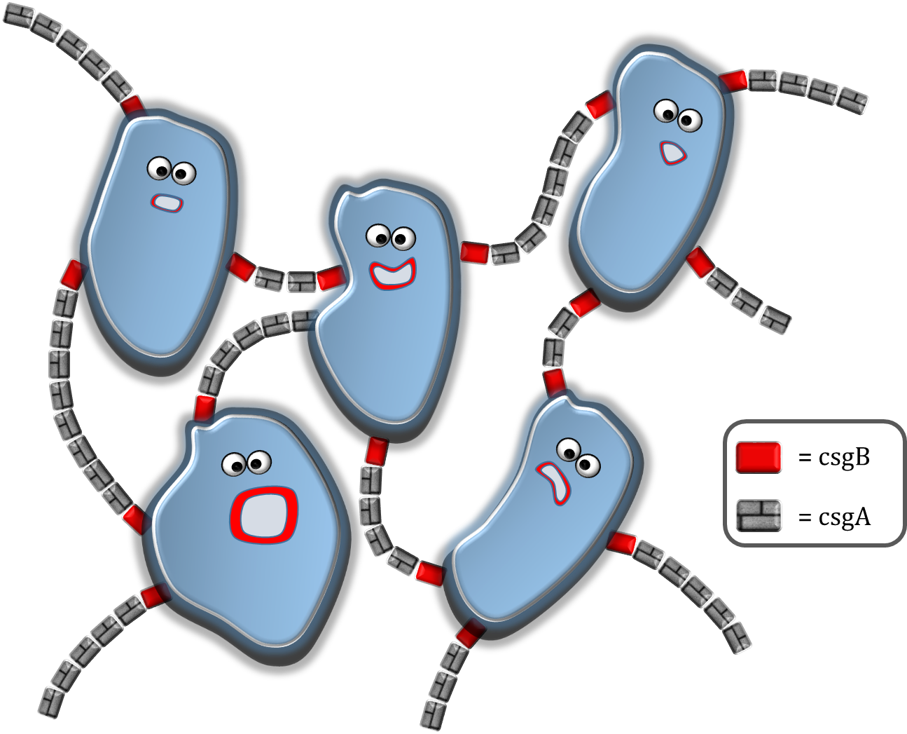
The activity of the promoter, denoted as PoPs, can be calculated by a kinetic experiment with GFP. For this experiment, we made a construct with GFPmut3 (modified GFP variant with stronger fluorescent signal) and csgA under the same rhamnose promoter. The constructs used for this experiment are depicted in Fig. 2.


As csgA and GFP are under the same promoter, the fluorescence of GFP can be related to the production of csgA. It is presumed that the promoter activity is independent of the addition of the GFPmut3 gene.
As already mentioned in the section “Kinetic experiment” under “Project”, both the fluorescence and OD600 were measured. It is important to also measure the cell density, as we are interested in the fluorescence per cell per second. To calculate how much fluorescence corresponds to a certain amount of GFP (in nanogram), a calibration curve has been constructed with wtGFP. As the ratio of emission maxima for GFPmut3 relative to wtGFP is 21 at an excitation of 488nm (Brendan et. al), the correct mass amount of GFP mut3 could be determined.
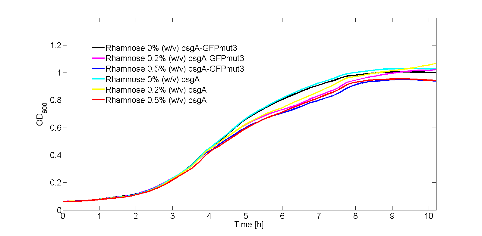
In Fig. 3, the OD600 is plotted for each of the samples in the kinetic experiment. As can be seen from Fig. 3, there is some difference in OD600 between the samples. Therefore, the fluorescence signal normalized by the number of cells as shown in Fig. 4:
In Fig. 3, the OD600 is plotted for each of the samples in the kinetic experiment. As can be seen from Fig. 3, there is some difference in OD600 between the samples. Therefore, the fluorescence signal normalized by the number of cells as shown in Fig. 4:
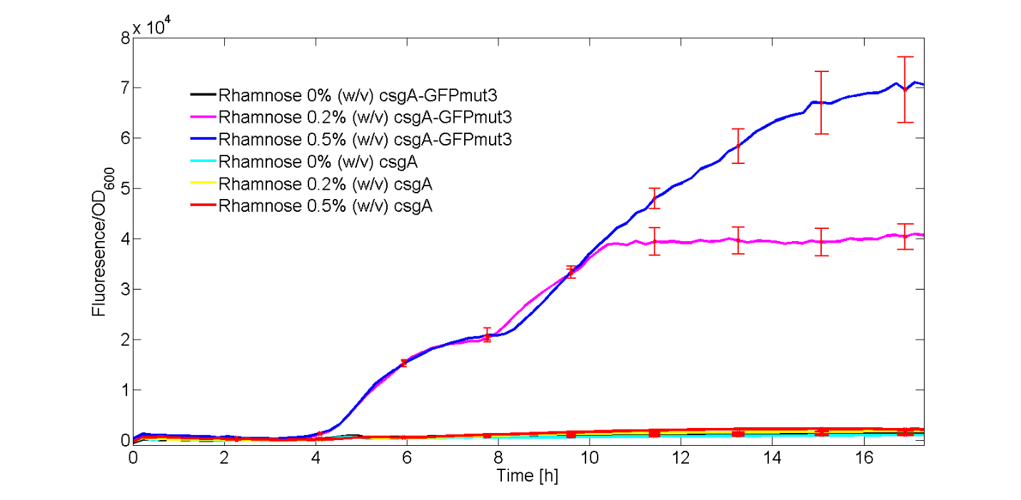
As can be seen from Fig. 4, GFPmut3 only appears if the culture has been induced by rhamnose. Furthermore, it can be seen that a higher induction level of rhamnose leads to an increase in GFPmut3 and thus fluorescence. Finally, as the fluorescence signal is normalized by the cell density, one can make statements about the activity of the rhamnose promoter. The promoter seems to not be active right after induction, but more after 3 or 4 hours. This is in accordance with data from literature (Wegerer et. al), in which a low amount of fluorescence with a rhamnose promoter was observed after 2 hours of induction.
The calibration line of fluorescence versus mass amount GFPmut3 is given in Fig. 5.
corresponding function of the GFPmut3 calibration line with massGFP in ng is:

With the calibration line, which was made with the exact same settings as the kinetic experiment, the mass amount of GFPmut3 per cell can be calculated. With Eq. 1, the fluorescence signal was converted to mass amount of GFPmut3 for rhamnose induction of 0.2% (w/v) and 0.5% (w/v).
After this conversion, the units are still in nanogram per OD600. As the desired unit is molecules per cells, the following dimension analysis has been performed:

The result of this unit conversion is shown in Fig. 6:
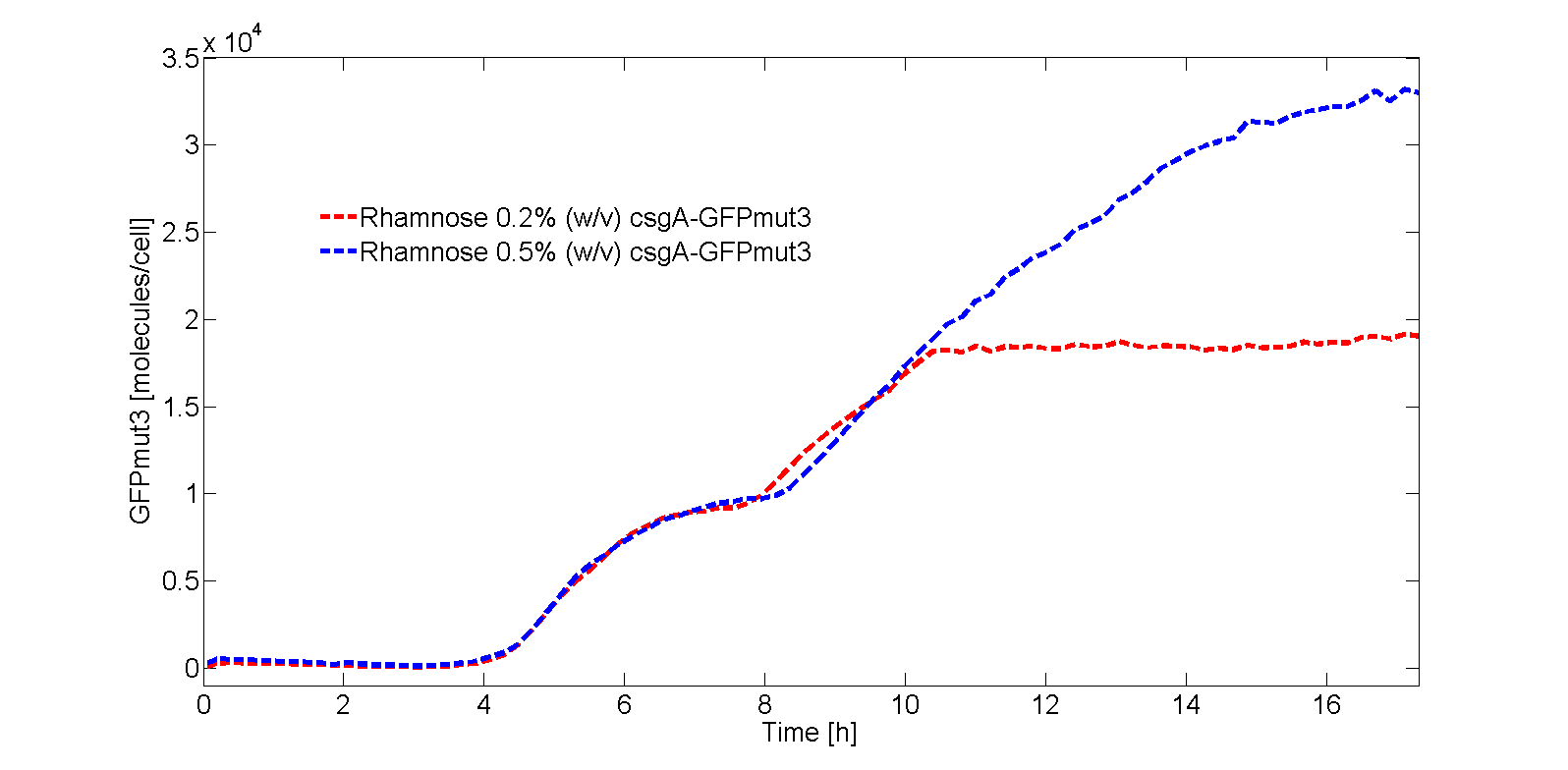
The GFPmut3 steady state concentrations are thus:

As the data is now converted to molecules per cell, it is possible to construct a model with the purpose of predicting the same steady state levels as in the performed experiments. The only unknown remaining in this model is the promoter activity, which can be varied to correctly fit the data.
The model that was made is a mathematical model of ordinary differential equations (ODE’s) describing the GFP mRNA concentration (Eq. 2), immature GFP protein concentration (Eq. 3) and mature GFP protein concentration (Eq. 4) in Table 1. All concentrations are modeled per cell per second. The immature protein is the nonfluorescent GFP, the mature protein is the fluorescent protein (which will be fitted to the data).


In the kinetic model, the growth rate of the bacteria is not a constant (as can be seen from Fig. 3). The bacteria grow exponentially from 2 to 3. 5 hours before going into the stationary phase. Until 2 hours, the bacteria are in the lag phase of growth. This growing behavior, in the order lag phase - exponential phase - stationary phase, is characterized with the following differential equation (Koseki et al.):
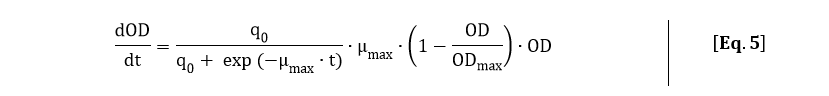
In order to fit Eq. 5 to the OD600 data depicted in Fig. 3, Eq. 5 was solved analytically:
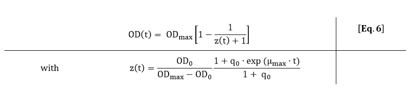
From Eq. 6, the parameters ODmax, q0 and µmax can be fitted to the OD600 data depicted in Fig. 3.
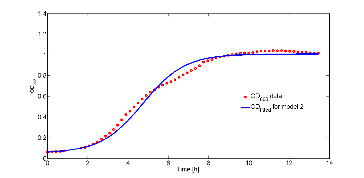
The fit of Eq. 6 to our OD600 data is shown in Fig. 7. As the OD600 profiles of rhamnose induction with 0.2% (w/v) and 0.5% (w/v) were similar, only the OD600 profile for 0.2% (w/v) was fitted to Eq. 6.
The fitted values for ODmax, q0 and µmax are:


From the fitted function of the OD600, an analytical expression for the growth rate can be derived. The growth rate is equal to:
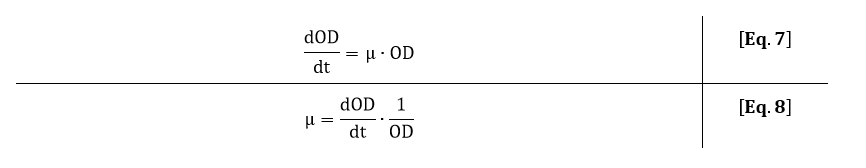
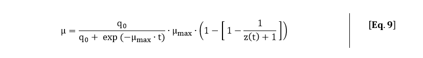
Filling in Eq. 7 and Eq. 8 in Eq. 9 gives the following expression for the growth rate:
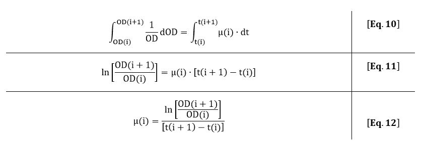
The growth rate can also be estimated from the OD600 by integrating Eq. 7:
In Fig. 8, the fitted growth rate as a function of time and the growth rate estimated from our data are both plotted.
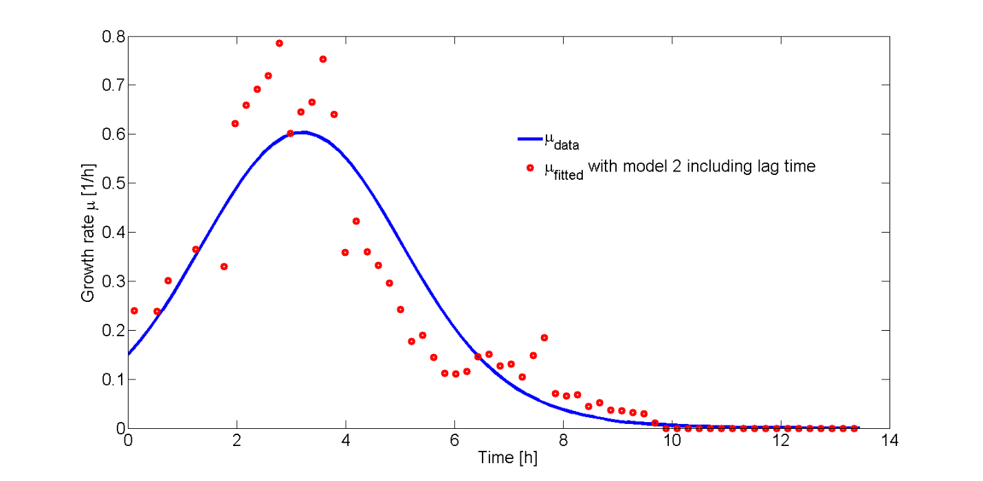
The difference between data and model can be explained by the approximation of the growth rate from the data or the error in the measurement of the plate reader. However, the growth rate function correctly describes the trend of the data.
csgA intracellular concentration
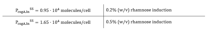
From the kinetic experimental data, the steady state concentration of GFP was 1.9∙104 molecules per cell for 0.2% (w/v) rhamnose induction and 3.3∙104 molecules per cell for 0.5% (w/v) rhamnose induction. As the csgA is transported to the extracellular space, the intracellular concentration of csgA (steady state) is not expected to be higher than the steady state concentration of GFP. Therefore, we estimate the steady state intracellular csgA concentration to be half the steady state concentration of GFP.
The intracellular steady state concentrations of csgA are thus:
In order to calculate the csgA concentration in and outside the cell, a system of ordinary differential equations (ODE) needs to be defined. This model is similar to the GFP ODE system, except that the csgA is transported out of the cell. As the transporter protein (csgG) is not ATP dependent (van Gerven et. al), it can be presumed that the rate of csgA transport is dependent on the intracellular csgA concentration times a transport rate constant (kt). Furthermore, the translation rate of csgA is higher than the GFP translation rate. The translation rate of csgA is equal to:

The system of ODE’s describing csgA intracellular and extracellular concentration can be found in Table 2.
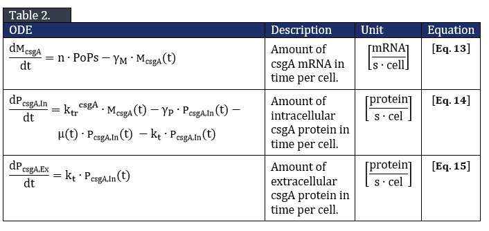

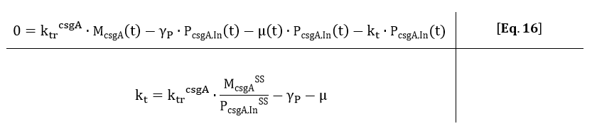
From Eq. 14, the steady state concentration of csgA can be calculated. As in steady state the accumulation of intracellular csgA is zero, the csgA transport rate can be written as:
From the kinetic model, the PoPs was fitted to our data and can be used to calculate the steady state concentration of csgA mRNA:
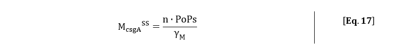
Filling in the steady state concentration of csgA mRNA gives:
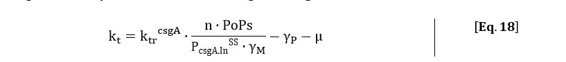
The degradation of csgA mRNA is presumed to be equal to the degradation of GFPmut3 mRNA. Furthermore, when the concentration of intracellular csgA has reached steady state, the growth rate of the culture will be close to zero as the culture will be in the stationary phase. Filling in the numbers in Eq. 18, gives a csgA transport rate constant of:

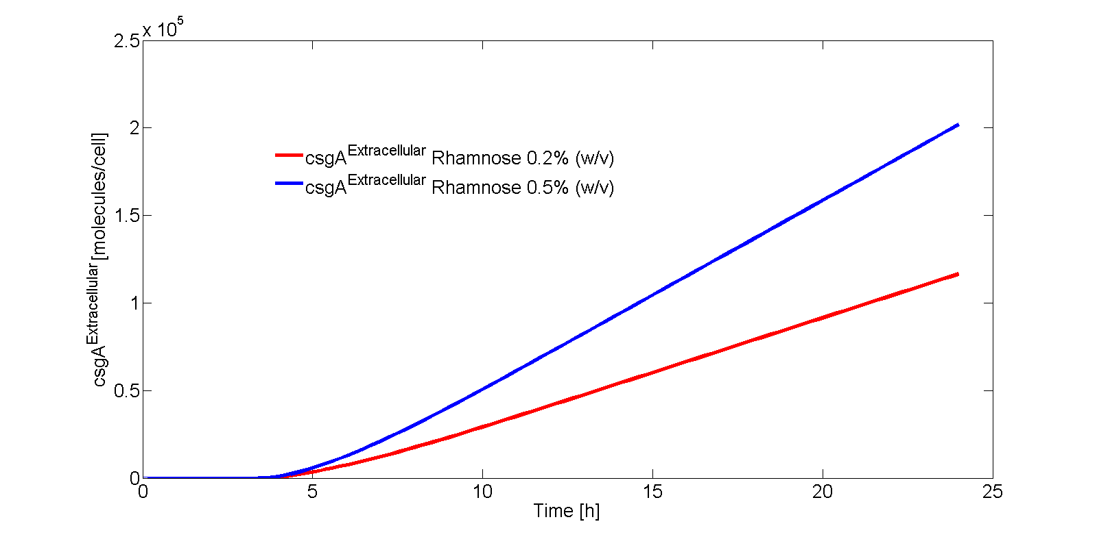
The extracellular csgA concentration can now be plotted as a function of time (Fig. 9).
If the intracellular concentration of csgA has reached steady state, the production of csgA is equal to:
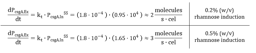
The extracellular concentration of csgA is thus equal to:
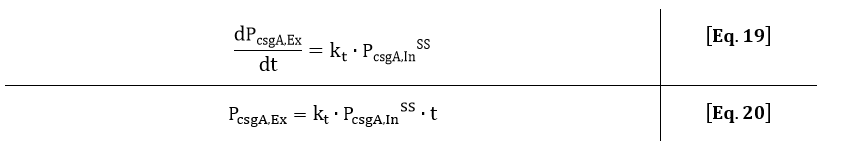
As can be seen from Eq. 20, if the intracellular concentration of csgA has reached steady state, the extracellular concentration of csgA will increase linearly in time (as can be also seen after 5 hours in Fig. 9).
As the production rate of csgA is in the order of 2-3 proteins per second, the csgA production will be limiting. This is because the number of csgB proteins in the outer membrane is more in the order of 100-1000 proteins csgB (Wang et. al). A higher induction level of rhamnose will produce more curlis, leading to a higher degree of curli intercellular connectivity and thus to a stronger biofilm. Therefore, with our inducible rhamnose promoter it is possible to control, to a certain degree, the biofilm strength of our printed samples.
Back to TopCurli Formation


Biofilm Strength
Subtitle or summary goes here. Should be short - two or three sentences.


Time for Printing


References
“FACS-optimized mutants of the green fluorescent protein (GFP)”, Brendan P. Cormack, Raphael H. Valdivia and Stanley Falkow, Gene, 173 (1996) 33-38
“Automated Live Cell Imaging of Green Fluorescent Protein Degradation in Individual Fibroblasts”, Michael Halter, Alex Tona, Kiran Bhadriraju, Anne L. Plant, John T. Elliott, Cytometry Part A ,71A: 827-834, (2007)
“Optimization of an E. coli L-rhamnose-inducible expression vector: test of various genetic module combinations”, Angelika Wegerer, Tianqi Sun and Josef Altenbuchner, BMC Biotechnology 2008, 8:2
https://greenfluorescentblog.wordpress.com/tag/gfpmut3/, (2012)
“Measuring the activity of BioBrick promoters using an in vivo reference standard”, Jason R Kelly, Adam J Rubin, Joseph H Davis, Caroline M Ajo-Franklin, John Cumbers, Michael J Czar, Kim de Mora, Aaron L Glieberman, Dileep D Monie and Drew Endy, Journal of Biological Engineering 2009, 3:4
“Alternative Approach To Modeling Bacterial Lag Time, Using Logistic Regression as a Function of Time, Temperature, pH, and Sodium Chloride Concentration”, Shige Koseki and Junko Nonaka, FEMS Yeast Res 14 (2014) 586–600
“Gatekeeper residues in the major curlin subunit modulate bacterial amyloid fiber biogenesis”, Xuan Wang, Yizhou Zhou, Juan-Jie Ren, Neal D. Hammer, and Matthew R. Chapman, PNAS, (2010), vol. 107., no.1, 163-168
http://parts.igem.org/Part:BBa_K914003
Secretion and functional display of fusion proteins through the curli biogenesis pathway, Van Gerven N, Goyal P, Vandenbussche G, De Kerpel M, Jonckheere W, De Greve H, Remaut H, Molecular Microbiology (2014) 91(5), 1022–1035