Difference between revisions of "Team:KU Leuven/Modeling/Internal"
| Line 689: | Line 689: | ||
<br> | <br> | ||
<br> | <br> | ||
| − | <img id="totcellBON src="https://static.igem.org/mediawiki/2015/e/e6/KUL_IM_SIM_CB_TDON.png" alt="Simulation of all processes in Cell B in ON" style="width:100%;height:100%"> | + | <img id="totcellBON" src="https://static.igem.org/mediawiki/2015/e/e6/KUL_IM_SIM_CB_TDON.png" alt="Simulation of all processes in Cell B in ON" style="width:100%;height:100%"> |
<br> | <br> | ||
<br> | <br> | ||
Revision as of 17:52, 17 September 2015

Internal Model
1. Introduction
We can think of many relevant questions when implementing a new circuit: how sensitive is the system, how much will it produce and will it affect the growth? As such, it is important to model the effect of the new circuits on the bacteria. This will be done in the Internal Model. We will use two approaches. First we will use a bottom-up approach. This involves building a detailed kinetic model with rate laws. We will use Simbiology and ODE's to study the sensitivity and dynamic processes inside the cell. This is the bottom-up approach. Afterwards, a top-down model, Flux Balance Analysis (FBA), will be used to study the steady-state values for production flux and growth rate. This part is executed by the iGEM Team of Toulouse as part of a collaboration and can be found here
2. Simbiology and ODE
In the next section we will describe our Simbiology model. Simbiology allows us to calculate systems of ODE's and to visualize the system in a diagram. It also has options to make scans for different parameters, which allows us to study the effect of the specified parameter. We will focus on the production of leucine, Ag43 and AHL in cell A and the changing behavior of cell B due to changing AHL concentration. In this perspective, we will make two models in Simbiology: one for cell A and one for cell B. First we will describe how we made the model and searched for the parameters. Afterwards we check the robustness of the model with a parameter analysis and we do scans to check for the effects of molecular noise.
3. Quest for parameters
We can divide the different processes that are being executed in the cells in 7 classes: transcription, translation, DNA binding, complexation and dimerization, protein production kinetics, degradation and diffusion. We went on to search the necessary parameters and descriptions for each of these categories. To start making our model we have to chose a unit. We choose to use molecules as unit because many constants are expressed in this unit and it allows us to drop the dillution terms connected to cell growth. We will also work with a deterministic model instead of a stochastic model. A stochastic model would show us the molecular noise, but we will check this with parameter scans.
The next step is to make some assumptions:
- The effects of cell division can be neglected
- The substrate pool can not be depleted and the concentration (or amount of molecules) of substrate in the cell is constant
- The exterior of the cell contains no leucine at t=0 and is perfectly mixed
- Diffusion happens independent of cell movement and has a constant rate
4. System
After this extensive literature search, we can finally set up our complete system of ODEs for every cell.
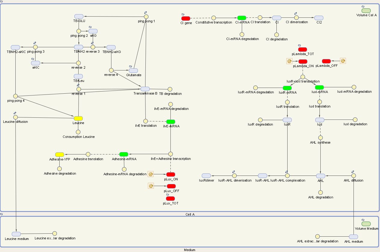
The designed circuit in Cell A is under control of a temperature sensitive cI repressor. Upon raising the temperature, cI will dissociate from the promoter and the circuit is activated. This leads to the initiation of the production of LuxR and LuxI. LuxI will consecutively produce AHL, which binds with LuxR. The newly formed complex will then activate the production of Leucine and Ag43. Leucine and AHL are also able to diffuse out of the cell into the medium. Ag43 is the adhesine which aids the aggregation of cells A, while Leucine and AHL are necessary to repel cells B.
We can extract the following ODE's from this circuit:
Cell A equations
Symbols:${}$ ${\alpha}$: transcription term, ${\beta}$: translation term, $d$: degradation term,
$D$: diffusion term, ${ K_d}$: dissociation constant, n: Hill coefficient, L: leak term
$$\frac{{\large d} m_{cI}}{d t} = \alpha_1 {\cdot} cI_{gene} - d_{mCI} {\cdot} m_{cI}$$ \begin{align} \frac{{\large d}{cI}}{d t} = \beta_{cI} {\cdot} {m_{cI}} -2 {\cdot} {k_{cI,dim}} {\cdot} {cI}^2 + 2 {\cdot} {k_{-cI,dim}}{\cdot} {[cI]_2} - d_{cI} {\cdot} {cI} \end{align} $$\frac{{\large d}{[cI]_2}}{d t}= k_{cI,dim} {\cdot} {cI}^2 - {k_{-cI,dim}}{\cdot} {[cI]_2} $$ $$\frac{{\large d} m_{LuxI}}{d t} = (L_{lambda} + {\frac{\alpha_{lambda}}{1 + ({\frac{[cI]_2}{K_{d1}}})^{n_{cI}}}}) {\cdot} LuxI_{gene} - d_{mLuxI} {\cdot} m_{LuxI} $$ $$\frac{{\large d} m_{LuxR}}{d t} = (L_{lambda} + {\frac{\alpha_{lambda}}{1 + ({\frac{[cI]_2}{K_{d1}}})^{n_{cI}}}}) {\cdot} LuxR_{gene} - d_{mLuxR} {\cdot} m_{LuxR} $$ $$\frac{{\large d} LuxI}{d t} = \beta_{LuxI} {\cdot} {m_{LuxI}} - d_{LuxI} {\cdot}{LuxI} $$ $$\frac{{\large d} LuxR}{d t} = \beta_{LuxR} {\cdot} {m_{LuxR}} -k_{lux,as} {\cdot}{LuxR}{\cdot}{AHL_{in}} + k_{lux,dis}{\cdot}{[LuxR/AHL]} - d_{LuxR} {\cdot}{LuxR} $$ $$\frac{{\large d} AHL_{in}}{d t} = {k_{luxI}} {\cdot} {luxI} - k_{lux,as} {\cdot}{luxR}{\cdot}{AHL_{in}} + k_{lux,dis}{\cdot}{[luxR/AHL]}+ ( {D_{IN,AHL}} {\cdot} {AHL_{out}} - {D_{OUT,AHL}} {\cdot} {AHL_{in}} ) - d_{AHL,in} {\cdot} {AHL_{in}} $$ $$\frac{{\large d} AHL_{out}}{d t} = ( {D_{OUT,AHL}} {\cdot} {AHL_{in}} - {D_{IN,AHL}}{\cdot}{AHL_{out}} ) -d_{AHL,out}{\cdot}{AHL_{out}} $$ $$\frac{{\large d} [luxR/AHL]}{d t} = k_{lux,as} {\cdot}{luxR}{\cdot}{AHL_{in}} - k_{lux,dis}{\cdot}{[luxR/AHL]} - 2 {\cdot} k_{lux,dim} {\cdot}{[luxR/AHL]^2} + 2 {\cdot}{k_{-lux,dim}}{\cdot}{[luxR/AHL]_{2}} $$ $$\frac{{\large d} [luxR/AHL]_{2}}{d t} = k_{lux,dim} {\cdot}{[luxR/AHL]^2} - k_{- lux,dim} {[luxR/AHL]} $$ $$\frac{{\large d} m_{ilvE}}{d t} = (L_{lux} + \frac{\alpha_{lux}}{1+(\frac{K_{d2}}{[luxR/AHL]_{2}})^{n_{lux}}} ) {\cdot} ilvE_{gene} - d_{milvE} {\cdot} {m_{ilvE}} $$ $$\frac{{\large d} m_{Ag43}}{d t} = (L_{lux} + \frac{\alpha_{lux}}{1+(\frac{K_{d2}}{luxR/AHL]_{2}})^{n_{lux}}} ) {\cdot} Ag43_{gene} - d_{mAg43} {\cdot} {m_{Ag43}} $$ $$\frac{{\large d} Ag43}{d t} = \beta_{Ag43} {\cdot} {m_{Ag43}} - d_{Ag43} {\cdot} {Ag43} $$ $$\frac{{\large d} Transaminase B}{d t} = \beta_{TB} {\cdot} {m_{ilvE}} - kf_1 {\cdot} {Transaminase B} {\cdot}{Glutamate} + kf_{-1}{\cdot}{[TB-GLU]} - kr_1 {\cdot}{Leucine_{in}}{\cdot}{Transaminase B} + kr_{-1}{\cdot}{TB-Leu} + kcat2{\cdot}{[{TBNH}_2-aKIC]} + kcat4{\cdot}{[{TBNH}_2-aKG]} + k_{production} - d_{TB} {\cdot} {Transaminase B}$$ \begin{align} \frac{{\large d}{TB}}{d t}= & \beta_{TB} {\cdot} {m_{ilvE}} - {kf}_{1}{\cdot}{TB}{\cdot}{Glu} + {kf}_{-1}{\cdot}{[TB-GLU]} - {kr}_1{\cdot}{Leucine}_{in}{\cdot}{[TB-GLU]} \\\\ & + {kr}_{-1}{\cdot}{[TB-Leu]} + {kcat2}{\cdot}{[{TBNH}_2-aKIC]} + {kcat4}{\cdot}{[{TBNH}_2-aKG]} - d_{TB}{\cdot}{TB} \end{align} $$\frac{{\large d}{[TB-GLU]}}{d t}= -{kcat1}{\cdot}{[TB-GLU]} + {kf}_{1}{\cdot}{TB}{\cdot}{Glu} - {kf}_{-1}{\cdot}{[TB-GLU]} $$ \begin{align} \frac{{\large d}{[{TBNH}_2]}}{d t}= & {kcat1}{\cdot}{[TB-GLU]} + {kcat3}{\cdot}{[TB-Leu]}- {kf}_{2}{\cdot}{{TBNH}_2}{\cdot}{aKIC} + {kf}_{-2}{\cdot}{[{TBNH}_2-aKIC]} \\\\ & - {kr}_2{\cdot}{{TBNH}_2}{\cdot}{aKG} +{kr}_{2}{\cdot}{[{TBNH}_2-aKG]} \end{align} $$\frac{{\large d}{[{TBNH}_2-aKIC]}}{d t}= -{kcat2}{\cdot}{[{TBNH}_2-aKIC]} + {kf}_{2}{\cdot}{{TBNH}_2}{\cdot}{aKIC} - {kf}_{-2}{\cdot}{[{TBNH}_2-aKIC]} $$ $$\frac{{\large d}{[TB-Leu]}}{d t}= {kr}_1{\cdot}{Leucine}_{in}{\cdot}{[TB-GLU]} - {kr}_{-1}{\cdot}{[TB-Leu]} - {kcat3}{\cdot}{[TB-Leu]} $$ $$\frac{{\large d}{[{TBNH}_2-aKG]}}{d t}= {kr}_2{\cdot}{{TBNH}_2}{\cdot}{aKG} - {kr}_{2}{\cdot}{[{TBNH}_2-aKG]} - {kcat4}{\cdot}{[{TBNH}_2-aKG]}$$ $$\frac{{\large d}{Leucine_{in}}}{d t}= {kcat2}{\cdot}{[{TBNH}_2-aKIC]} - {kr}_1 {\cdot}{Leucine_{in}}{\cdot}{Transaminase B} + {kr}_{-1}{\cdot}{[TB-Leu]} - d_{Leu}{\cdot}{Leucine_{in}} - {D_{OUT,Leu}}{\cdot}{Leucine_{in}} + {D_{IN,Leu}}{\cdot}{Leucine_{out}}{\cdot}\frac{{V_{cell}}}{V_{external,leu}} $$ $$\frac{{\large d} Leucine_{out}}{d t} = (D_{OUT,Leu} {\cdot}{leucine_{in}} - D_{IN,Leu} {\cdot}{leucine_{out}}) - d_{Leu,out} {\cdot} {Leucine_{out}} $$
We visualize these ODE's in the Simbiology Toolbox which results in the following diagram:
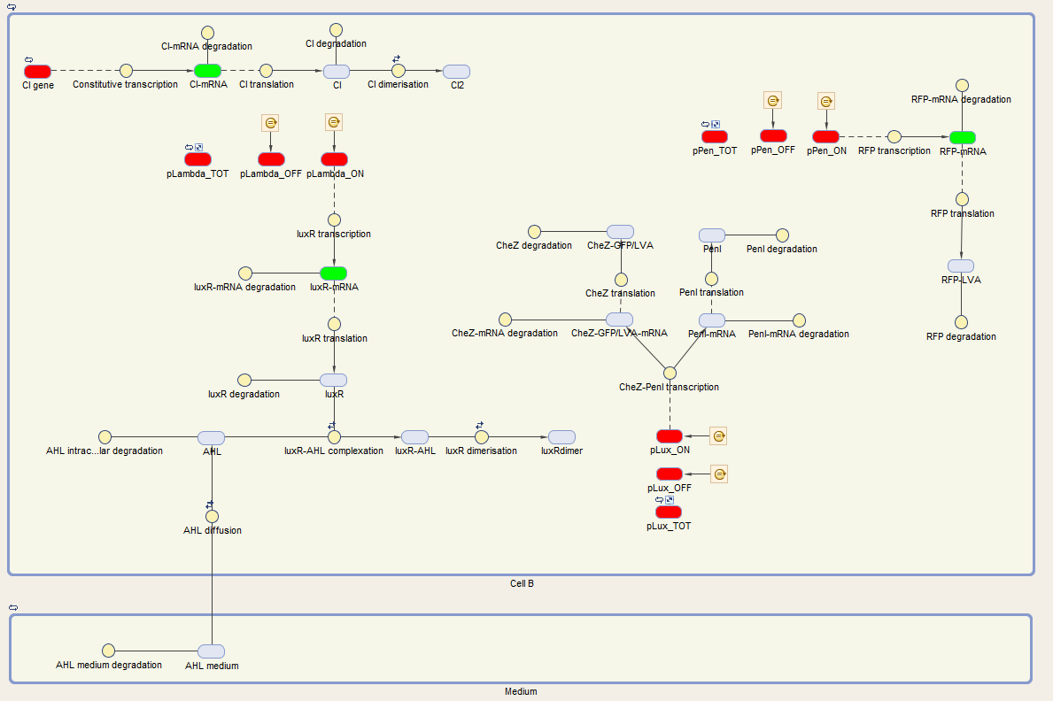
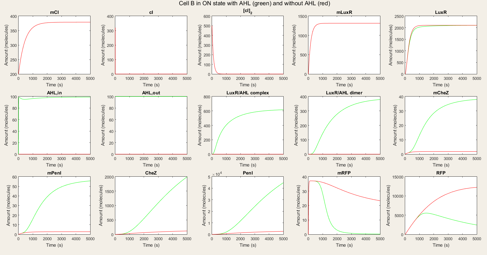
The system of Cell B is also under control of the cI repressor and is activated similar as cell A. The activation by the temperature raise, leads to the production of LuxR. AHL of the medium can diffuse into the cell, binding LuxR and activating the next component of the circuit. This leads to the production of CheZ and PenI. CheZ is the protein responsible for cells to make a directed movement, governed by the repellent Leucine. PenI is a repressor which will shut down the last part of the circuit which was responsible for the production of RFP.
We can extract the following ODEs for Cell B from this sytem:
Cell B equations
Symbols: ${\alpha}$:transcription term, ${\beta}$:translation term, $d$:degradation term,
$D$:diffusion term, ${ K_d}$:dissociation constant, n:Hill coefficient, L:leak term
$$\frac{{\large d} m_{cI}}{d t} = \alpha_1 {\cdot} cI_{gene} - d_1 {\cdot} m_{cI}$$ $$\frac{{\large d}{cI}}{d t} = \beta_1 {\cdot} {cI} -2 {\cdot} {k_{cI,dim}} {\cdot} {cI}^2 + 2 {\cdot}{k_{-cI,dim}}{\cdot} {[cI]_2} - d_{cI} {\cdot} {cI} $$
We visualize these ODE's in the Simbiology toolbox. This gives us the following diagrams:
5. Results
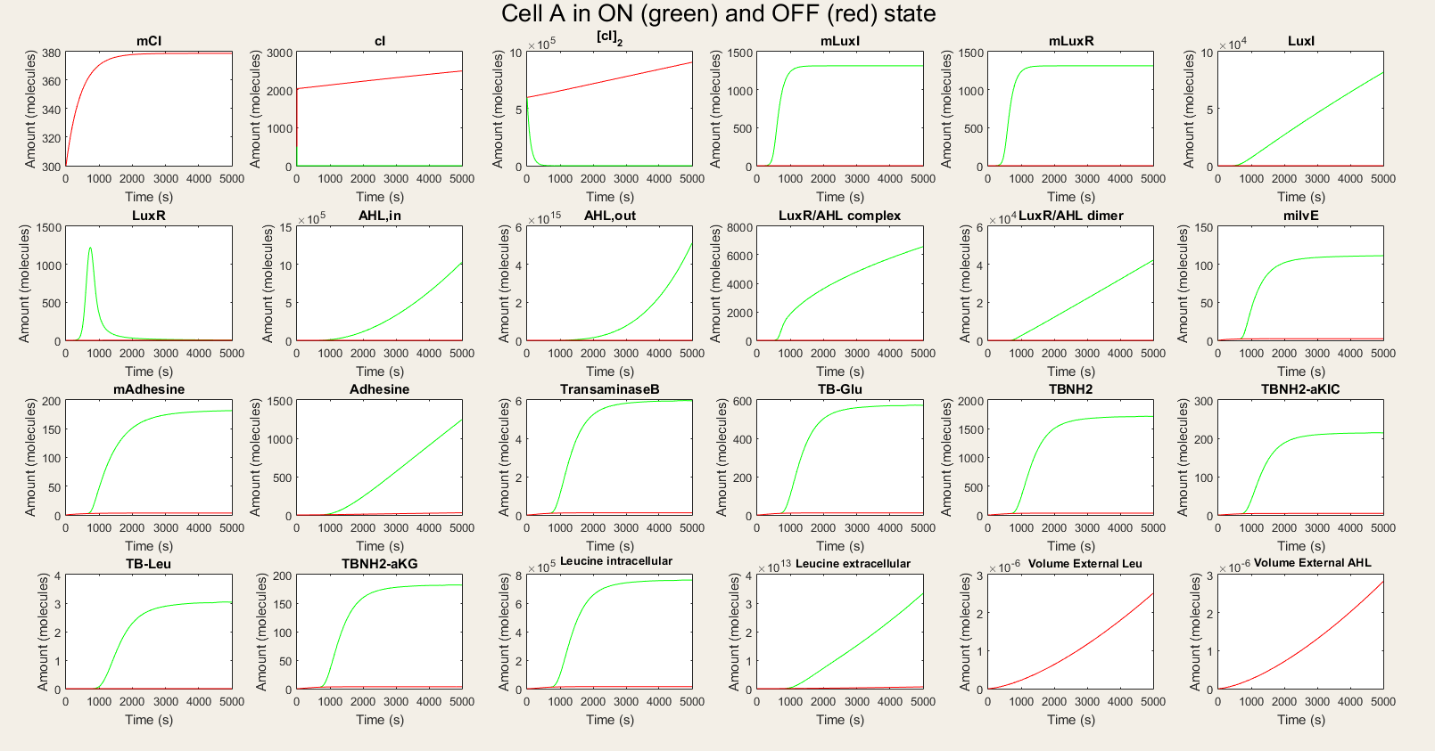
For cell A we made a simulation with cell A in the ON mode as visuable in figure (x). To do this we had to disable the sensitive cI-repressor. This was done by increasing the value of the degradation rate of the repressor. This will be visuable in our simulation because cI gets to 0 fairly quick. We also see that after a while all the LuxR proteins are bound to AHL. Some values are really big (for example the dimer, AHL, Leucine and LuxI values are really high. This is all possible because we do not account for the metabolic burden that is put on the cell in producing these biomolecules. For studying this effect we used FBA. The most interesting we can learn of this graphs is that the cell works according to our design.
Cell A graph of all, graph of Leucine, graph of AHL
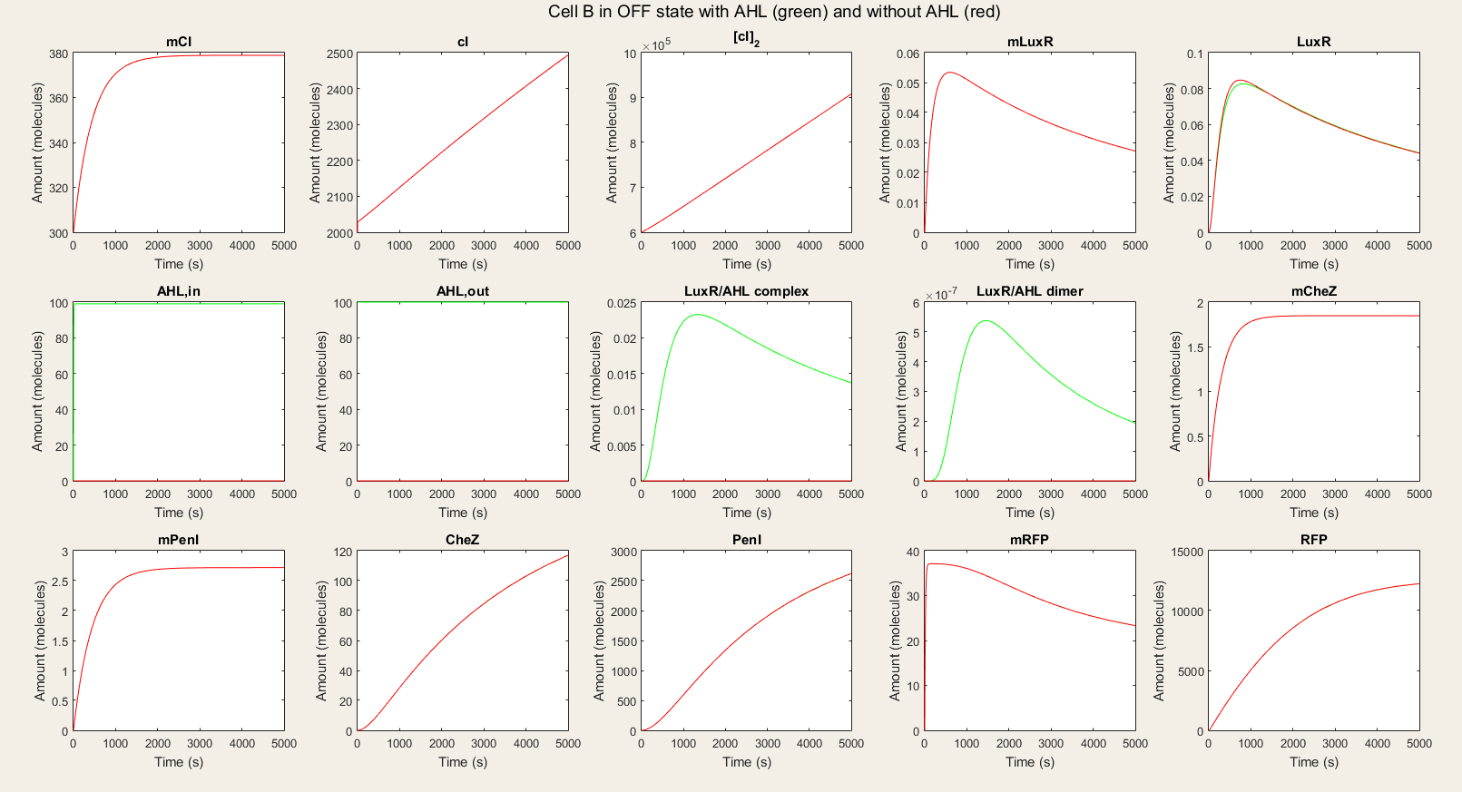
Cell B graph of all, graph with induction and without induction
Sensitivity analysis
Conclusion and discussion


