Team:KU Leuven/Modeling/Toulouse

Toulouse FBA Model
We cooperated with Toulouse on the modeling. Here we describe the Flux Balance Analysis the Toulouse team generously
performed for us.
Flux Balance Analysis is a widely used approach for studying the flow through metabolic networks. In our
case we are interested in the leucine and AHL production rates of the type A cells and their effect on the growth rate of the bacteria. This is very important because if cell A has a big metabolic burden and thus, a very low growth rate, cell B would overgrow it and our pattern formation system would not work. Therefore, it is very important to keep the growth rates of cells A and cells B as close as possible to each other. To check the effect of our system on the growth rate iGEM Toulouse ran a FB analysis.
When a FBA is set up. The metabolic network of the organism in question is represented as a matrix $\mathbf{S}$
of size $m \times n$ . This matrix is filled with the stoichiometric constants of each reaction. Each of the $m$ matrix
rows represents a unique compound. Similarly each of the n columns represents one unique reaction. Next
a vector $\mathbf{v}$ of length $n$ is defined which contains the flux through each reaction. Finally, the
vector $\mathbf{x}$ is defined to contain the concentrations of each metabolite. The steady state solution
is the insteresting one, therefore:
$$ \frac{dx}{dt} = \mathbf{Sv} = 0 $$
Which is the nullspace of $\mathbf{S}$. In this set of solutions, a maximal or minimal value can be identified
using numerical optimization. In order to run the optimization algorithm a cost function has to be defined.
$$ f(x) = \mathbf{c}^{T}\mathbf{v} $$
The equation above shows such a cost function. Here the vector $\mathbf{c}$ represents a weight vector. In practice
it is used to choose the metabolite of interested by setting the corresponding entry to one and all others to zero.
From an optimization perspective the equation $\mathbf{Sv} = 0$ represents constraints, which guide the numerical
solver to the right solution.
In our case the $\mathbf{S}$ matrix comes from the in silico E. coli model K-12 MG1665. The model is contained in an XML file.
We told the Toulouse modelers our two reaction of interest:
$$ \text{glutamate} + \text{aKIC} \rightarrow \text{aKG} + \text{Leucine} $$
This reaction is interesting as leucine serves as repellent in our scheme. The second reaction of interest is:
$$ \text{acylACP} + \text{SAM} \rightarrow \text{ACP} + \text{MTA} + \text{AHL} $$
This reaction is important because AHL serves as the key to the motility system of cell B. Without AHL, cell B is unable to move away from cell A and form patterns.
Given this information the Toulouse team was able to locate the reactions of interest in the XML model file,
and simulate the cell metabolism. The results are shown in figures 1 and 2. All of the graphs shown above are in $mmol \cdot gDW^{-1} \cdot h^{-1}$. In figure 1 the effect of AHL production on growthrate was plotted and in figure 2 the effect of leucine production. We can also deduce the maximum possible flux of AHL and leucine. This is the flux that corresponds to a growth rate of 0. In our case these maximum values are:
For AHL: $ 150.71391 mmol \cdot gDW^{-1} \cdot h^{-1}$
For leucine: $ 528.17774 mmol \cdot gDW^{-1} \cdot h^{-1}$
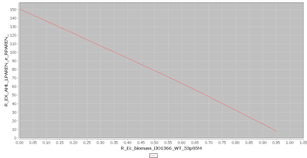
Figure 1
AHL and Biomass production. Click to enlarge
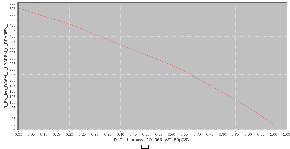
Figure 2
Leucine and Biomass production. Click to enlarge
Yet, we are interested in the combined effect of AHL and leucine production on the growth rate. This is why Toulouse also modeled the effect of one biomolecule, but with the constraint that the other biomolecule is produced at maximum rate. The results of these simulations are shown in figures 3 and 4. We see that the production values are way smaller in this simulation. This is logical, since more resources are being used. It is impossible to reach the maximum production rates, while producing two biomolecules.
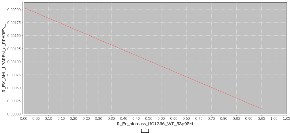
Figure 3
AHL and Biomass production with maximal Leucine production rate. Click to enlarge
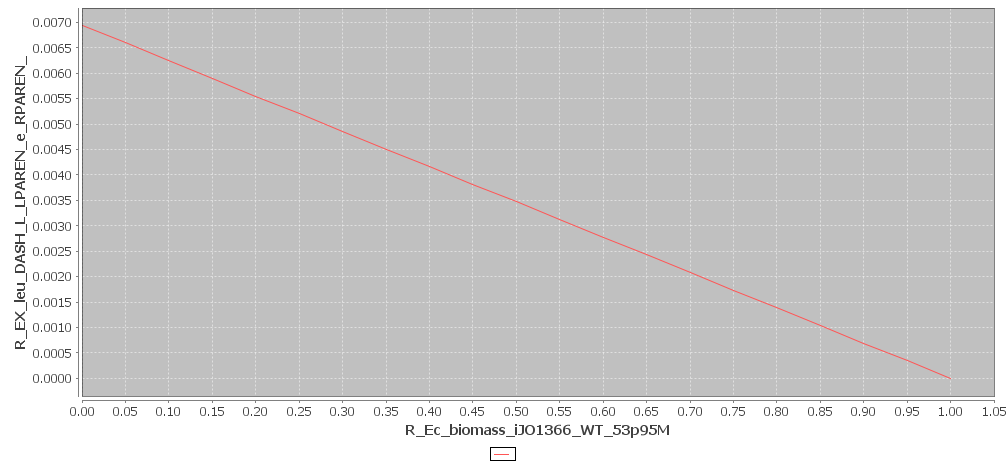
Figure 4
Leucine and Biomass production with maximal production rate. Click to enlarge
In generally it follows from the analysis that the more AHL or leucine is produced the smaller the biomass output becomes. It also shows that cell A can not operate at the maximum production rate, because the growth rate would then be so slow that cell B would overgrow it. This is something to keep in mind when we choose our promoters for the system. If our promoters are too strong, the growth rate of cell A will be too low and cell B will be able to overgrow cell A.


Contact
Address: Celestijnenlaan 200G room 00.08 - 3001 Heverlee
Telephone: +32(0)16 32 73 19
Email: igem@chem.kuleuven.be


