Team:KU Leuven/Modeling/Top
1-D continuous model
The biological circuit described on the
Research page is going to be modelled. Two different cell types A and B are interacting.
Type A cells produce a repellent called leucine which causes
the cells of type B to move away. At the same time, type A cells also produce AHL, which is required by the cells of type
B to move. Initially, colonies of the two bacteria types are placed
at the center of the dish. As molecule production within the type A cells kicks in, the repellent and AHL concentrations
start to increase. This triggers the type B cells to move away from the center. Movement will continue until the
concentration of AHL is insufficient for the type B cells to move further. The behaviour of the two cell types
is described by the model given below:
Our Keller-Segel type model
$$\frac{\partial A}{\partial t} = D_a \bigtriangledown^2 A + \gamma A(1 - \frac{A}{k_{p}}),$$ $$\frac{\partial B}{\partial t} = D_b \bigtriangledown^2 B + \bigtriangledown (P(B,H,R) \bigtriangledown R) + \gamma B(1 - \frac{B}{k_{p}}), $$ $$ \frac{\partial R}{\partial t} = D_r \bigtriangledown^2 R + k_r A - k_{lossH} R $$ $$\frac{\partial H}{\partial t} = D_h \bigtriangledown^2 H + k_h A - k_{lossR} H . $$With:
$$ P(B,H,R) = \frac{B K_{c} H}{R}. $$
The model has been derived while looking at [1] and [2]
.
The terms that appear can be grouped into four categories. Every equation has a diffusion term given by
$D_x \bigtriangledown^2 X$, diffusion smoothes peaks by spreading them out in space. The two equations related to cell
densities contain logistic growth terms of the form $\gamma X(1-\frac{X}{k_x})$, which model the cell growth during
simulation time. Finally the second equation describing the moving cells comes with a variable coefficient Poisson term
$\bigtriangledown (P \bigtriangledown X)$ which describes the cell movement. Last but not least,
we have the two bottom equations. These two model concentrations.
Both contain linear production and degradation terms, which look
like $kX$. It is important to keep in mind that even though the degradation terms appear as linear terms in the
differential equation the solution will be exponential decay.
To generate the video file, the system has been discretized using a finite volume approach in conjunction,
with an explicit Euler scheme. For finite volume methods to work, we rewrote our equations as conservation laws. Then each
grid point is assigned the area around it, such that flux of cells or molecules leaving one cell enters another one. From
discretizing the integrated conservation law the following expression is obtained in one dimension:
Discretized Keller-Segel type model
$$ A^{n+1}_j = A^n_j + \triangle t \cdot (D_a/(\triangle x)^2 \cdot ( A^n_{j-1} + A^n_{j+1} - 2 \cdot A^n_j)) ... $$ $$ + \gamma \cdot A^n_j \cdot (1 - A^n_j / kp)) $$ $$B^{n+1}_j = B^n_j +\triangle t \cdot (1/ (\triangle x)^2 \cdot (D_b\cdot (B^n_{j-1} + B^n_{j+1} - 2B^n_j)\dots $$ $$ +(P^n_{j+\frac{1}{2}} \cdot (R^n_{j+1} - R^n_j) - P^n_{j-\frac{1}{2}} \cdot (R^n_j - R^n_{j-1}))) \dots $$ $$ + \gamma \cdot B^n_j \cdot (1 - B^n_j / kp)) $$ $$ R^{n+1}_j = R^n_j + \triangle t \cdot( D_r \cdot (R^n_{j+1} + R^n_{j-1} - 2 R^n_j) /(\triangle x^2) \dots $$ $$ + kr \cdot A^n_j - k_{lossR} \cdot R^n_j) $$ $$ H^{n+1}_j = H^n_j + \triangle t \cdot ( D_h \cdot (H^n_{j+1} + H^n_{j-1} - 2 H^n_j) / (\triangle x)^2 \dots $$ $$ + k_h \cdot A^n_j - k_{lossH} \cdot H^n_j ) $$For the equations given above, the left hand side values at the next time step depend exclusively on data of the previous time step as illustrated in the figure below:
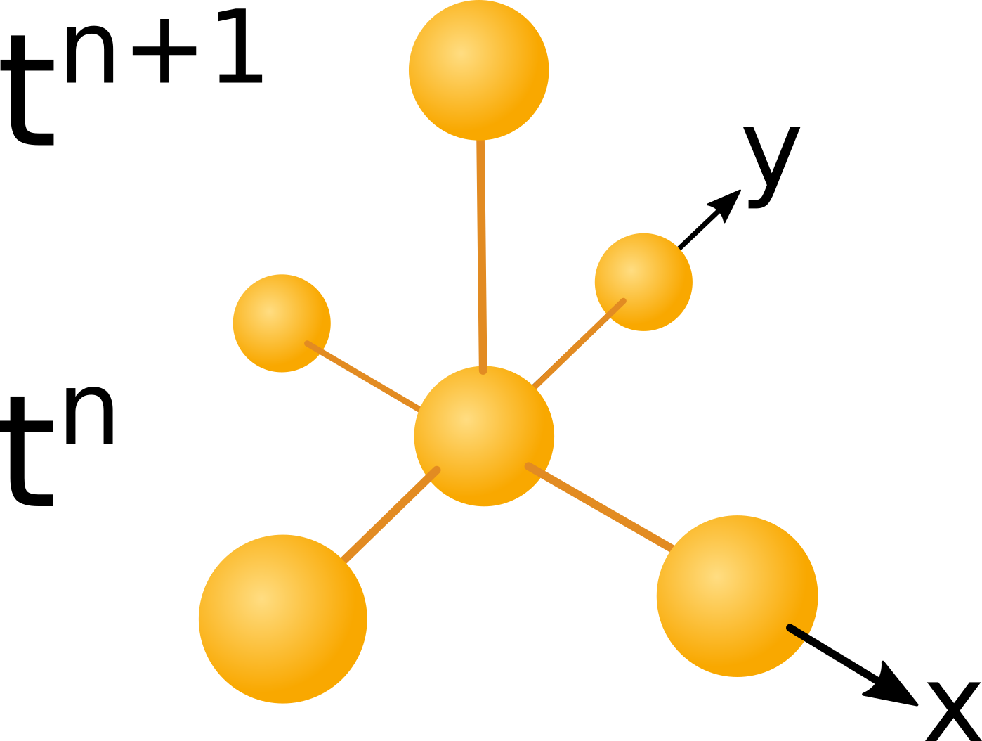
Figure 1
Computational molecule. Click to enlarge
The image above shows the dependency of data in time and space. The computational molecule used in this case utilizes only
data of the previous time level $t_n$ to compute data at the next time level $t_{n+1}$. A scheme with a space time
dependency like the one shown above is called an explicit scheme.
The video box above shows the solution of the discretized system in one dimension. To gain additional insight into the
effect of the different terms of the model, we computed simulations of different term combinations. Use the buttons
to choose from the videos.
The first term in each equation is a diffusion term. Diffusion smooths out edges of an initial condition, eventually
it leads to an even distribution. The initial condition in the diffusion simulation is rectangular the illustrate the
smoothing. Another important part of the two first equations which model bacteria density is the logistic growth term.
The video which visualizes logistic growth starts with a Gaussian distributed initial condition, which is more realistic
then the rectangular initial condition used in the diffusion term simulation.
The most important term is the chemotaxis term $\bigtriangledown (P(B,H,R) \bigtriangledown R)$. It is simulated in conjuction
with diffusion. The evening out of the diffusion term leads to acceptable solutions throughout a wider parameter range.
However, the result shown in the video is not satisfactory. No chemicals are simulated, the assumption here is that the type
B cells are directly repelled by type A bacteria, apart from the problem that this is biologically impossible the resulting
wave is quite small and would probably not be recognizable on a Petri dish. The next step we took was to use a model closer
to what is possible in nature and include the repellent leucine in the simulation. An additional simulation including logistic
growth with a high growth constant ($\gamma = 0.008$) and leucine production can be played by clicking the corresponding
button above.
This simulation shows that high bacterial growth rates are quite detrimental to pattern formation.
Another video with a lower growth constant ($\gamma = 0.002$) shows more promising results, but the wave could be more
pronounced. The last simulation can be played above.
This one included leucine and AHL it is thus equivalent to the Keller-Segel type model shown in the first box
and the discretization provided in the second box. Hereby, including AHL which increases cell motility at the center of the
plate where the colonies are initially placed the model to produces a satisfactory large wave.
Fortunately the reproduction rate can be adjusted by choosing the temperature or the growth medium accordingly, therefore
it should be possible to achieve the low growths needed for pattern formation in the lab.
Zero flux and periodic boundary conditions have been implemented. The boundaries are the edges of the domain on which the
equation system is solved. Here the domain ranges from zero to eight centimetres, which is the diameter of a Petri dish.
With zero flux boundaries
the first derivative is set to zero at the boundaries, which means that neither bacteria nor chemicals are allowed to pass
trough the boundary. Periodic boundaries connect pairs of boundaries to each other, which means that cells leaving at the top
of the boundary appear at the bottom,
cells leaving at the left boundary reappear at the right and so on. In the continuous context these boundary conditions have
been implemented to allow comparisons with the hybrid model, where these boundaries are also used.
Finally simulations have been done using the parameters given in the table below:
| Parameter | Value | Unit | Source | Comment |
|---|---|---|---|---|
| $D_a$ | $0.072 \cdot 10^{-3}$ | $cm^2/h$ | following [1] | |
| $D_b$ | $2.376 \cdot 10^{-3}$ | $cm^2/h$ | following [1] | |
| $D_r$ | $26.46 \cdot 10^{-3}$ | $cm^2/h$ | as found in [6] | $298.2 K$ |
| $D_h$ | $50 \cdot 10^{-3}$ | $cm^2/h$ | from [3] | |
| $K_{c}$ | $8.5 \cdot 10^{-3}$ | $cm^2 \cdot cl/h$ | estimated | |
| $\gamma$ | $0.002$ | $h^{-1}$ | estimated | |
| $k_p$ | $1.0 \cdot 10^3$ | $cl^{-1}$ | estimated | |
| $k_h$ | $17.9 \cdot 10^{-4}$ | $fmol/h$ | computed from [4] and [8] | |
| $k_r$ | $5.4199\cdot 10^{-4}$ | $fmol/h$ | computed from [7] and [8] | |
| $k_{lossH}$ | $ln(2)/48$ | $h^{-1}$ | from [5] | $ ph = 7$ |
| $k_{lossR}$ | $ln(2)/80$ | $h^{-1}$ | estimated |
2-D continuous model
Using the equation system as described above, the model may also be simulated in two dimensions. Once more a finite volume approach has been taken in connection with an explicit Euler scheme. All parameters have been kept constant with the one exception of the chemotactic sensitivity $K_c$. This has been increased to $K_c = 1.5 * 10^{-1} cm^2/h$ and therefore leads to earlier pattern formation. Above four simulation videos with Gaussian initial conditions can be observed. A fifth video shows a simulation using random initial data. The two last videos illustrate the effect of zero flux and periodic boundary conditions.
References
| [1] | D. E. Woodward, R. Tyson, M. R. Myerscough, J. D. Murray, E. O. Budrene, and H. C. Berg. Spatio-temporal patterns generated by Salmonella typhimurium. Biophysical journal, 68(5):2181-2189, May 1995. [ DOI | http ] |
| [2] | Benjamin Franz and Radek Erban. Hybrid modelling of individual movement and collective behaviour. Lecture Notes in Mathematics, 2071:129-157, 2013. [ http ] |
| [3] | Monica E Ortiz and Drew Endy. Supplement to- 1754-1611-6-16-s1.pdf, 2012. [ .pdf ] |
| [4] | A. B. Goryachev, D. J. Toh, and T. Lee. Systems analysis of a quorum sensing network: Design constraints imposed by the functional requirements, network topology and kinetic constants. In BioSystems, volume 83, pages 178-187, 2006. [ DOI ] |
| [5] | A. L. Schaefer, B. L. Hanzelka, M. R. Parsek, and E. P. Greenberg. Detection, purification, and structural elucidation of the acylhomoserine lactone inducer of Vibrio fischeri luminescence and other related molecules. Bioluminescence and Chemiluminescence, Pt C, 305:288-301, 2000. |
| [6] | Tatsuya Umecky, Tomoyuki Kuga, and Toshitaka Funazukuri. Infinite Dilution Binary Diffusion Coefficients of Several α-Amino Acids in Water over a Temperature Range from (293.2 to 333.2) K with the Taylor Dispersion Technique. Journal of Chemical & Engineering Data, 51(5):1705-1710, September 2006. [ DOI ] |
| [7] | Xuejing Yu, Xingguo Wang, and Paul C. Engel. The specificity and kinetic mechanism of branched-chain amino acid aminotransferase from Escherichia coli studied with a new improved coupled assay procedure and the enzyme's potential for biocatalysis. FEBS Journal, 281(1):391-400, January 2014. [ DOI ] |
| [8] | Yasushi Ishihama, Thorsten Schmidt, Juri Rappsilber, Matthias Mann, F Ulrich Hartl, Michael J Kerner, and Dmitrij Frishman. Protein abundance profiling of the Escherichia coli cytosol. BMC genomics, 9:102, 2008. [ DOI ] |


Contact
Address: Celestijnenlaan 200G room 00.08 - 3001 Heverlee
Telephone: +32(0)16 32 73 19
Email: igem@chem.kuleuven.be


