Team:Cambridge-JIC/Measurement
Camera Specifications
| pixel size: | 1.4μmx1.4μm |
| sensor size: | 2592x1944 pixels |
| total: | 5MP |
| focal length: | 3.6mm |
| aperture: | 1.25mm |
Resolution Assessment of a Microscope Based on a Raspberry Pi Camera
Theory of Optics
The resolution can be limited by two independent factors:
pixel size;
diffraction effects.

The larger of these determines the actual limitation of the system. In our case we know that the pixel size is 1.4 μm, so we now need to work out the diffraction limit, that is the smallest spot size which can be produced by the lens with the given specs. To calculate this, recall the Rayleigh criterion for a circular aperture: sinθ=1.22 λ/d. Here λ~550nm is the wavelength of light, taking green for the middle of the visible spectrum, d=1.25mm is the diameter of the aperture and θ (small angle) is the angular radius of the spot, that is tanθ=r/L. Here r is the radius of the spot projected at a distance L from the aperture, which in our setup is actually the focal length f of the Raspberry Pi camera lens (and the spot is projected onto the CCD sensor).
From first approximation for a small angle: sinθ=tanθ, so 1.22 λ/d=r/f. Rearranging this equation and plugging in the numbers gives the following diameter of the smallest resolvable spot: 2r=3.8μm. This is almost three times the size of the pixel on the CCD, which imposes the actual limit on the resolution. The pixels of the CCD outresolve the theoretical lens limits.
Final resolution estimate of a microscope based on Raspberry Pi camera: 3.8μm

Compare this with a typical size of a chloroplast: 5-8μm diameter [1]. Our resolution will be just enough to image them, which is exactly what we have managed to do on this picture of Spirogyra cells. Note that these are larger than typical chloroplasts though. To obtain a better resolution, a lens with either larger aperture and/or shorter focal distance can be used, without the need of a better CCD. However, this is a tradeoff in terms of worse aberration and contrast. An improvement to the resolution will however be required in order to image bacteria, for example, which are of the order of 1μm in diameter [2].
[1] Wise, R. and Hoober, J. (2006). The structure and function of plastids. Dordrecht: Springer.
[2] Encyclopedia Britannica, (2015). bacteria :: Diversity of structure of bacteria. [online] [Accessed 30 Jul. 2015].
Inverting the Lens: Why and How
The way a camera works is by focusing an image of a distant large object as a small set of points onto the CCD, which is positioned close to the lens (in its focal plane). Theoretically however, it might as well do the opposite (because light paths are reversible – a well known and intuitive physical principle): that is, inspect the CCD pixels and project their greatly enlarged image onto a distant screen.
The lens has a small aperture (1.25mm) at one end, and a larger one (4mm) offering a wider view angle at the other, which is required for viewing close up objects. This is normally oriented towards the CCD.


So, if we want to image a sample on a microscope slide, we need to:
position the lens close to the sample – at roughly the focal distance, that is 3.6mm;
orient the lens with its larger aperture towards the sample;
position the sensor behind the lens, now at a much larger distance (roughly 2.8cm) – for this we have designed a special camera mount.
Now we have the Raspberry Pi camera working as a microscope!
The problem: how to unscrew the lens from the camera The Raspberry Pi camera is sold with the lens screwed (and lightly glued) into the sensor casing. To unscrew the lens, you will need the right type of pliers: ideally with ridged surface. Grip the top part of the plastic casing of the lens firmly, being careful not to crush it, and rotate counterclockwise. After the first small rotation, you should be able to unscrew it fully manually. ATTENTION: might not work from the first time! Do not try to cut out the lens or force it out in any other way.
3D Printed Material Testing
Comparison of Typical 3D Printer Materials [1]
Acrylonitrile Butadiene Styrene (ABS):It is strong, flexible, with good machinability and a higher temperature resistance. These properties can make it more popular for use in professional applications. It’s plastics petroleum based origin cause it to have a less pleasant hot plastic smell. The 3D printer requires a heated print bed for use with ABS.
Polylatic Acid (PLA):Its wide range of colours and translucencies make it attractive to many. It has plant based origins giving it a sweet smell. When it is properly cooled, PLA can have higher max printing speeds, sharper printing of corners and thinner layers. It also has low warping on printed parts making it a popular plastic for use in 3D printing.
Standard Material Properties
| Material Property |
PLA |
ABS |
|---|---|---|
| Density (Mg/m3) | 1.25 | 1.01-1.21 |
| Young’s Modulus E (GPa) | 3.5 | 1.1-2.9 |
| Elongation at break (%) | 6 | 3-75 |
| Melting (softening) temperature Tm (oC) | 160 | 88-128 |
| Glass Transition Temperature (oC) | 60 | 100 |
| Yield Stress σy (MPa) | - | 18.5-51 |
| Tensile Strength σts (MPa) | 36-55 | 25-50 |
| Thermal expansion (μm/m-K) | - | 83-95 |
| Strength to weight ratio (kN-m/kg) | 40 | 31-80 |
Table 1: Material properties of PLA and ABS [2][3][4]
Makerbot Material Properties Chart
| Material Property |
PLA |
ABS | ||
|---|---|---|---|---|
| Standard (STD) | High Resolution (MAX) | Standard (STD) | High Resolution (MAX) | |
| Impact Strength (Un-notched) IZOD* (J/m) | 96.1 | 219 | 304 | 331 |
| Compressive Strength (peak) (MPa) | 17.9 | 93.8 | 7.6 | 49 |
| Tensile Strength (peak) (MPa) (MPa) | 46.8 | 65.7 | 34 | 38.1 |
| Flexural Strength (peak) (MPa)(MPa) | 61.8 | 94.7 | 36.8 | 59.6 |
Table 2: Makerbot material properties chart for PLA and ABS [5]
*IZOD impact testing is a standard method of determining the impact resistance of materials. The results are expressed in energy lost per unit of thickness (such as ft·lb/in or J/cm) at the notch.
Experimental Testing: Instron Machine 3-point Bending
Introduction


Figures 1 and 2: Test 1 and Test 3 in position within the instron machine at the start of loading.
The Instron Machine is a commercial testing machine which is widely used in industry for characterising materials. The material is simply supported on rollers and a load cell applies a force to its centre (fig.1 and 2). A continuous force is applied until the material fails under the load. A force against deflection (of load cell) graph is plotted which allows the Young’s modulus (E) of the material to be calculated using equation 1.
E=kL3/4bd3
Equation 1: k=gradient of linear part of force-deflection graph, L=distance between supports, b=width of sample, d=thickness of sample
Method: Material Preparation
Beams of length 100mm (thickness 3mm, 1mm) and 150mm (thickness 0.8mm, 1mm and 3mm) were used for a three point bending test.
Printing for 100mm beams: Makerbot, PLA
Printing for 150mm beams: Ultimaker 2, PLA
Infill: 20%
Layer resolution: 0.2mm
Print speed: 50mm/s
Travel speed:150mm/s
Print-bed temperature: 72˚C
Results

Figure 3: Graph of Applied Force against Crosshead Displacement during a Instron three point bend test.
Note: error bars are negligible on the graph, the instron machine is a standard commercial machine with high precision.

Figure 4: Regions of hysteresis carried out during three point bending test
| Sample |
Length (mm) |
Base (mm) | Thickness (mm) | Young’s Modulus (GPa) |
|---|---|---|---|---|
| 1: Makerbot, PLA | 100 | 20 | 3 | 2.47 |
| 2: Makerbot, PLA | 100 | 20 | 1 | 1.55 |
| 3: Ultimaker2, PLA (3D printed base side down) | 150 | 20 | 3 | 32.1 |
| 4: Ultimaker2, PLA (3D printed base side up) | 150 | 20 | 3 | 27.2 |
| 5: Ultimaker2: PLA | 150 | 20 | 1 | 31.1 |
| 6: Ultimaker2: PLA | 150 | 20 | 0.8 | 52.0 |
Table 3: Samples used in three point bending test with corresponding calculated Young’s Modulus value.
Failure Surfaces


Figures 5 and 6: Makerbot sample 1 (t=3mm) and Ultimaker sample 1 (t=3mm) at the end of three point bending test respectively.
Discussion
Comparison was made of samples 1 and 3, the two samples of 3mm thickness, with 1 made using the Makerbot and 3 made using the Ultimaker2 3D printing machines. It can be clearly seen in the graphs in fig.3 that sample 3 is the stronger sample, it can be loaded to ~4 times that of sample 1 before it begins to fail. The stiffness of sample 3 is ~13 times stiffer than sample 1 (E=32.1GPa compared to 2.47GPa).
There is also a difference in the way that the two samples fail under the applied load. With sample 1 it can be seen that the material cracks across the whole sample simultaneously. A brittle, clean fracture surface can be seen in fig. 5. This failure behaviour is also seen in the graph, where the applied load immediately falls to zero. In comparison to this sample 3 does not actually crack by the end of the test. As can be seen in fig. 6 the cracks try to propagate along the diagonal strips of material, but this orientation prevents the crack from spreading to the edge of the material, and so it tries to propagate along the other direction, producing the zigzag pattern shown. No crack is formed, the material is just elongated at the point of load, weakening the material. The difference in the failure of these two samples is due to the way in which the samples are built up during printing. Both are built from the bottom in alternating layers of oppositely oriented strips of material. The Makerbot lays down horizontal and vertical layers while the Ultimaker2 creates diagonal strips of material, increasing its strength.
Sample 3 and 4 are the same sample tested with the base of the 3D printed material facing down and facing up respectively. The sample with the base material facing down was found to be stronger. As the maximum bending will occur at the furthest side from the loading head, it is possible that the base material is strongest when it is printed facing onto the 70 degrees hot plate. This would allow for subsequent layers to melt into the first creating an intertwined lattice formation. As the layers build up further from the hot plate, this would be less likely to occur.
The thinner samples (samples 2, 5 and 6) find it hard to hold a load as they are so flexible and so a high enough load is never applied to cause failure. This method of high stress testing may not be ideal for such samples.
A hysteresis was carried out during each test as shown in fig. 4. This provided positive results for the use of the material within the microscope. It can be seen that as well as exhibiting linear behaviour on loading the material also unloads and reloads along approximately the same linear line. This shows that the material is not work hardened by bending under the small loads that it would be exposed to within the microscope. No plastic deformation is taking place that could lead to premature failure.
For sample 3 a drop can be seen in the graph and then the sample can be seen to be reloaded. This was due to the sample coming off its support during testing but then clicking back into place.
[1] Chilson, L. (2013). The Difference Between ABS and PLA for 3D Printing. [online] [Accessed Jul. 2015].
[2] Make It From (2015). Polylactic Acid (PLA, Polylactide). [online] [Accessed Jul. 2015].
[3] Make It From (2015). Acrylonitrile Butadiene Styrene (ABS). [online] [Accessed Jul. 2015].
[4] Cambridge Engineering Department (2003). Materials Databook. [online] [Accessed Jul. 2015].
[4] Makerbot PLA and ABS Strength Data. [online] [Accessed Jul. 2015].
Stage Drift Characterisation
Introduction
In order to perform time-lapse imaging, the digital microscope must be left capturing images for long periods of time. However, most microscope stages exhibit 'drift', which causes the sample to move during the experiment. This can seriously affect the results, and must be fully characterised before solutions are developed. The causes of drift are complex, and can be as a result of thermal expansion, mechanical movement and vibrations amongst other factors [1][2].
In order to characterise our prototype brightfield microscope, an experiment was set up to record the movement of points (fiducial mark) on a slide over a period of roughly 16 hours. This is an established technique for measuring drift [3]. A free, open-source video analysis and modelling software was used to manually track the points over time. Two key conditions were tested: the first was the normal working set-up, the second was carried out with the screws linking the translation knobs to the stage itself removed. This essentially uncouples the stage from the translation knobs, and the sample is then moved until it's in the correct orientation. The experimental objective was to characterise the movements of our 3D printed stage in isolation, and compare this to it's movements when coupled to the translation knobs as it would be when fully functional.
Methods
Time lapse set-up:
Raspberry pi camera set up to take images at 5 min intervals overnight
Used prototype brightfield microscope, with a standard micrometer slide (one major division = 100µm)
Code used is summarised here and is based on a standard Raspberry Pi camera tutorial
Movie creation and tracking
Used iMovie to compile still images into a single movie
A single point was tracked using Tracker software carried out over intervals of 20 frames across the entire time lapse
Calibration was achieved using the micrometer scale
The coordinate grid is arbitrary, and the origin was selected to be the starting point of the point being tracked (such that the drift path starts at roughly (0,0). The axes were orientated with respect to the alignment of the micrometer slide at the start of the test in both test
Note: tracking involves selecting the target point manually through the course of the time-lapse, which will introduce human error
Figure 1: Scale bar (dark blue) was used for calibration. Origin was initially centred on the point being tracked. Point being tracked is marked at t=0 (light blue circle). Axis and calibration bar were aligned with the micrometer scale by eye. In order to increase the accuracy of the tracking, a filter was used to convert the image to grayscale and the contrast was increased
Brightfield Test 1
In total it comprised of 203 images, taken every 5 minutes, displayed for 0.4s each
Discounted final image for movement speed calculations (No. 203), as this was taken after the slide have been moved slightly when we returned to the lab to check the results
Image tracking was repeated 4 times, and each time the x and y coordinates were recorded. This was an attempt to reduce the significance of human error in image tracking
The data were combined, and the averaged plotted with error bars indicating ± 1 SD
Brightfield Test 2
In order to test the effect of our translation system on drift, the screws connecting the stage to the translation knobs were removed. This was intended to test the mechanical effect of the attached screws on drift
201 images obtained using a time-lapse program, taken every 5 minutes, displayed for 0.4s each
Image tracking was repeated 4 times, and each time the x and y coordinates were recorded. This was an attempt to reduce the significance of human error in image tracking
The data were combined, and the averaged plotted with error bars indicating ± 1 SD
Comparison
The results from Test 2 were artificially shifted on the coordinate axis such that both paths start at the same original point (this modifies the results such that the starting position of the points being tracked are effectively the same, but the drift behaviour is different in each test)
The sole purpose of this translation was to plot the two graphs on the same axis in an informative way, to compare the paths of the two points under different conditions. This was necessary because the point tracked in each experiment were different, and therefore had different relative starting positions on the microscope slide
The movements of the starting point under two different conditions: screws attached (BT1), and no screws attached (BT2) were compared
BT1 based on 60,600 seconds of time-lapse (203 images). BT2 based on 60,000 seconds of time-lapse (201 images)
Results
The data from Brightfield Test 1 were aggregated


Figure 4: Graphs shows aggregated data from 4 trials in BT1. In all trials, the axis and calibration scale were consistent. Error bars indicate ± 1 SD
The data from Brightfield Test 2 were aggregated


Figure 5: Graph shows aggregated data from 4 trials in BT2. In all trials, the axis and calibration scale were consistent. Error bars indicate ± 1 SD
The data from Brightfield Tests 1 and 2 were then compared

Figure 6: Graph shows aggregated data from 4 trials in BT1 and in BT2 normalised of the same start point. Assumes points experience the same drift anywhere on the slide. In both trial groups, the axis and calibration scale were identical. They were not identical between BT1 and BT2. Error bars indicate ± 1 SD
Discussion
Results indicate that the attachment of the screws significantly reduces microscope drift compared to the stage with screws unattached
Results from BT2 suggest from the dynamics of the drift that the stage gradually approaches a stable equilibrium position
One potential solution may therefore be to determine the time taken to reach the equilibrium, and to image only once this has occurred
This will require further experimentation to determine whether the stage does actually reach a stable equilibrium, and how long this takes
However, with a fully motorised stage the screws must be attached, which changes the dynamics of the drift dramatically
Solutions have been proposed that make use of software to counteract drift using autofocus (for drift along z-axis). Additionally piezoelectric stages and automated stepper motors to actively remove drift (for movement along x-axis and y-axis) have also been implemented [3] [4]
In current fluorescent systems artificially labelled beads can be used as fiducial marks in the sample plane. Using a closed-loop feedback system, stage drift can then be corrected for based on the position of the fiduciary mark relative to the camera sensor [2]
Further testing, under different conditions such as different temperatures, will allow determination of the cause of drift when the screws are attached. However this is likely to be due to a number of factors each making a small contribution to overall stage movement.
[1] Microscopyu.com, (2015). Nikon MicroscopyU | Live-Cell Imaging | Focus Drift Correction. [online] [Accessed 10 Aug. 2015].
[2] Microscopedrift.com, (2015). Microscope Drift | The Solution to Focus Drift and Sample Drift. [online] [Accessed 10 Aug. 2015].
[3] Carter, A., King, G., Ulrich, T., Halsey, W., Alchenberger, D. and Perkins, T. (2007). Stabilization of an optical microscope to 0.1 nm in three dimensions. Appl. Opt., 46(3), p.421.
[4] Kreft, M., Stenovec, M. and Zorec, R. (2005). Focus-Drift Correction in Time-Lapse Confocal Imaging. Annals of the New York Academy of Sciences, 1048(1), pp.321-330.
Fact File
Battery
Want to do microscopy in the field? Or put your openScope inside a fridge? The great news is, openScope can run on battery for up to 12 hours. To power it up you will need to MoPi power module for Raspberry Pi and two 9V batteries. We recommend replacing the single 9V cell for a series of 6 1.5 AA batteries for best performance. For this purpose, you can 3D print this battery holder.
Cleaning
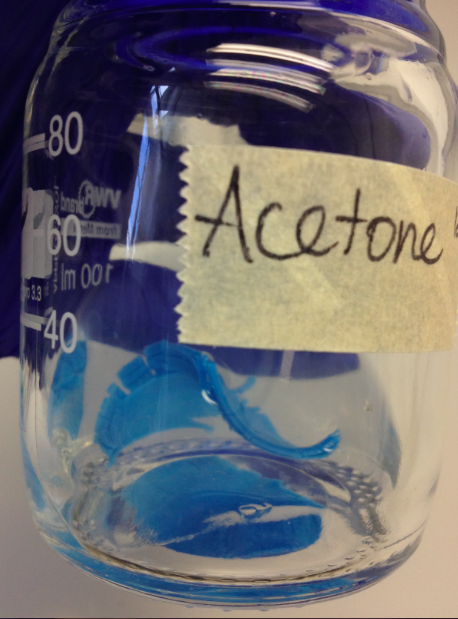
We are aware that an item put into your incubator can cause contamination and ruin your samples. Ugh. But this will not happen with openScope. Simply spray with isopropanol and it is ready! Isopropanol (a.k.a. propan-2-ol) is totally safe for the PLA and the electronics. Do not never ever attempt to use methanol (will make the PLA soft) or even worse, acetone (will simply destroy your microscope).