Team:Brasil-USP/interlabstudy
Interlab Study

2nd International InterLab Measurement Study in synthetic biology
In order to characterize standard biological parts, fluorescence-based assays have been widely used with a variety of fluorophores such as fluorescent proteins (FPs). Green fluorescent protein (GFP) is frequently applied as reporter gene to confirm gene expression and analyse its regulation. The Second International InterLab Measurement Study in synthetic biology proposes to detect three promoters activity by measuring and comparing the levels of GFP expression of three devices expressing GFP and controlled by one of the three promoters (see Figure 1). The three promoters - BBa_J23101, BBa_J23106, BBa_J23117 - are from the Anderson library (http://parts.igem.org/Promoters/Catalog/Anderson), a constitutive promoter family with different strengths.1

Figure 1: Interlab devices 1, 2 and 3, in order from top to down.
Introduction and Motivation
In the eleventh iGEM edition happens the second Interlab Study. This study is based on the characterization of standard biological parts and, as standard parts, it is fundamental to observe reproducibility and repeatability on their behaviour. For instance, even well characterized promoters in a given strain of E. Coli may behave reasonably different in another strain. Acknowledging this challenge, the Interlab Studies is a way to gather experiments from all around the world that only have one thing in common: the biological parts to be studied. Each research team has its own strains, plasmids and protocols. With this, we can construct a rich knowledge base of standard biological parts, together with several study cases of different protocols and other details. The value this have to the whole community of Synthetic Biology is beyond doubt.
We used a plate reader and a flow cytometer to measure fluorescence with biological and technical replicates, fulfilling InterLab study requirements and the extra credit. We evaluated the promoter strength of all devices using Relative Promoter Units [2] using DH5α E. Coli with backbone plasmid pSB1C3. Results show interesting differences: Device 2 (J23106) shows half the strength it would be expected in the original library.
Results
In the following subsections, we present our fluorescence measurements over time, a cytometry study showing a more microscopy view of how our cells behaved and our calculations of promoter strength using Relative Promoter Units (RPU). Notice that all of our data is publicly available here, and all software developed to calculate the results presented below are available here.
Sample definitions
We have three different samples from which we have used biological and technical triplicates. In the following we define each sample and the names we will use as reference throughout our text.
- Negative control (-control1) - cells with no plasmid, refering then to autofluorescence from DH5α E. coli cells. It was be used as baseline for our evaluations.
- Negative control (with plasmid) (-control2) - as a second negative control, DH5α E. coli cells containing a chloramphenicol resistant plasmid (pSB1C3) were used and no significant difference in the cells autofluorescence was detected when compared with wild DH5α E. coli cells
- Positive control (+control) - used the part I20270 in the pSB1C3 backbone (chloramphenicol resistant) was also measured.
- Device 1 (Dev1) - J23101 promoter with I13504.
- Device 2 (Dev2) - J23106 promoter with I13504.
- Device 3 (Dev3) - J23117 promoter with I13504.
Fluorescence results - plate reader
As described above, we have recorded fluorescence and optical density (OD) over time of a 96-well plate organized as mentioned before. We show below fluorescence measurements after 11h of experiments, when all colonies presented an OD of about 0.5 u.a., except of course LB and LB+Cam which do not have any bacteria. Notice that we have for three biological replicates of three technical replicates, as suggested for extra credit. If you are interested in our complete data, we have made it public here.

Table 1 (click for larger view): Fluorescence readings after 11h of experiment, not normalized by OD yet (see data below).
LB and LB+Cam are our baseline controls: they set the zero-level for the fluorescence. Although their levels are very close indeed, a Mann-Whitney U-statistic test showed that the antibiotic Cam is inducing a fluorescence that should not be disregarded (p-value < 0.5%). Thus, we will normalize all of our measures with respect to LB+Cam activity.
To better visualize this data, we show in the figure below The activity of each device averaged for each colony (considering the standard deviation). This fluorescence measure is normalized by LB+Cam. Notice how Device 3 fluorescence is close 1.0, i.e., not much is induced more than our zero-level activity. This is somehow expected, as this promoter is indeed very weak (see Relative Promoter Units below).

Figure 2 - Fluorescence per cell for each of the three colonies and for each device. While across colonies there is some difference, within the same colony the standard deviation is rather small. For all of our cases, Device 1 is the stronger promoter, followed by Device 2. Device 3 was always the weaker promoter.
The activity difference is definitely greater than the standard deviation of our measurements, guaranteeing our the hierarchy Device 1 > Device 2 > Device 3. We can see the time evolution of the fluorescence relative to the baseline control for each device.
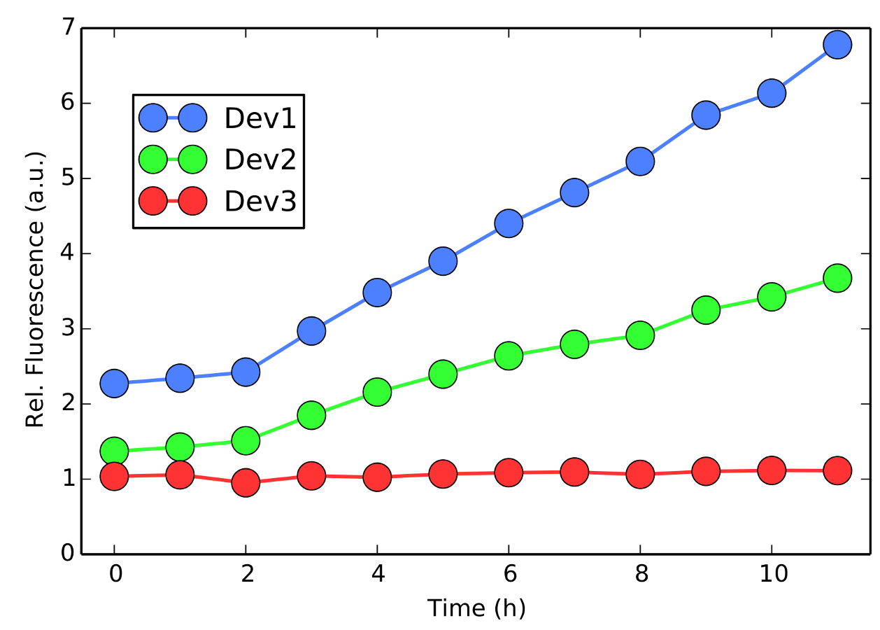
Figure 3 - Time evolution of the relative fluorescence per cell, normalized by the LB+Cam activity. All colonies are in their log-phase, suitable for evaluating their promoter strengths (see below). Notice that for all times, Device 1 is stronger than Device 2, while Device 3 is by far the weaker.
The figure above clearly shows that Device 1 induced significantly more activity. Still, Device 2 seems to perform better than Device 3. However, to quantitatively ensure that these activity differences are statistically relevant, we have performed a Mann-Whitney U-statistic test (p-value under 0.01%). Therefore, Device 1 is definitely stronger than Device 2, which in turn is also stronger than Device 3.
Cytometry
Here, we performed flow cytometry with biological triplicate. Because populations are well distinguished, quadrant gating method can be used to discern GFP expressing cells from those not expressing the GFP selection marker. FL1-H vs. FL2-H plots were divided in four quadrants - Q4 (lower left), Q3 (lower right), Q2 (upper left) and Q1 (upper right) - defined by analyzing negative control with no plasmid and fitting all events in the LL quadrant. Therefore, as FL1 detector (530/30 filter) collects green emission we obtained fluorescence intensity histograms for each sample, FL1-H vs. Counts.
Negative control (no plasmid)
Autofluorescence from DH5α E. coli cells and histogram markers FL1-H- and FL1-H+ were set, therefore, any event in the Q3 quadrant represents GFP fluorescence.

Figure 4 - E. coli DH5α cells. The cells were excited at 488 nm and detected using FL1-H (FITC channel). At the left, dot plot obtained by flow cytometry correspondent to autofluorescence whereby the lower left quadrant was defined to contain all cells as control. Histogram on the right shows autofluorescence levels. Both dot plot and histogram were used to set baseline and threshold.
Negative control (with plasmid)
Autofluorescence with chloramphenicol resistant plasmid.

Figure 5 - E. coli DH5α cells with chloramphenicol resistant plasmid pSB1C3 without insert DNA. The cells were excited at 488 nm and detected using FL1-H (FITC channel). At the left, dot plots obtained by flow cytometry correspondent to cells fluorescence and, at the right, histograms analysis of fluorescence levels.
Positive control

Figure 6 - E. coli cells GFP expression controlled by BBa_J23151 promoter. GFP was excited at 488 nm and detected using FL1-H (FITC channel). At the left dot plots obtained by flow cytometry correspondent to BBa_I20270 and histograms on the right show analysis of GFP expression in biological triplicate
Device 1

Figure 7 - E. coli cells GFP expression controlled by BBa_J23101 promoter. GFP was excited at 488 nm and detected using FL1-H (FITC channel). At the left dot plots obtained by flow cytometry correspondent to Device 1 (J23101 + I13504 ) and histograms on the right show analysis of GFP expression in biological triplicate
Device 2

Figure 8 - E. coli cells GFP expression controlled by BBa_J23101 promoter. GFP was excited at 488 nm and detected using FL1-H (FITC channel). At the left dot plots obtained by flow cytometry correspondent to Device 2 (J23106 + I13504 ) and histograms on the right show analysis of GFP expression in biological triplicate
Device 3

Figure 9 - E. coli cells GFP expression controlled by BBa_J23101 promoter. GFP was excited at 488 nm and detected using FL1-H (FITC channel). At the left dot plots obtained by flow cytometry correspondent to Device 3 (J23117 + I13504 ) and histograms on the right show analysis of GFP expression in biological triplicate
Comparison of expression rates of J23101, J23106 and J23117
Using flow cytometry we it is suggested that promoter strength decreases like J23101 > J23106 > J23117 (Device 1 > Device 2 > Device 3).

Figure 10 - Comparison of GFP expression controlled by BBa_J23101, BBa_J23106 and BBa_J23117 promoters. GFP was excited at 488 nm and detected using FL1-H (FITC channel).
Relative Promoter Units
According to the Anderson Promoter Collection [1], Device 1 should be stronger among the tested promoters in this experiment. Moreover, we can numerically measure a relative promoter strength and compare with the values available in the Anderson Collection. To measure then, we have to evaluate the following equation while our colonies are in the log-phase of their growth [2]:
\[ RPU_{\phi} = \frac{ \left\langle \frac{dF_{\phi}}{dt}\frac{1}{OD_{\phi}} \right\rangle }{ \left\langle \frac{dF_{J101}}{dt}\frac{1}{OD_{J101}} \right\rangle } \]
Notice that this measure is evaluated with respect to Device 1, thus we will be able to measure the promoter strength of devices 2 (J23106) and 3 (J23117). In compliance with the Anderson Collection, we set to 0.7 the promoter strength of the device 1 (J23101). All our colonies were in the log-phase (colocar figura!). See below our results, the expected values and the relative error.

We have also measured the promoter strengths of all controls to compare with the devices being tested, as shown below. We have normalized everything to Relative Promoter Units (RPU) using Device 1 as reference. As expected [2], different strains (and even chassis and plasmids) present different promoter strengths. Possibly, different protocols may also result in under- or over-expressing genes. Originally, most of experiments for Anderson's library were performed with W3110 strain (plasmid pSB3K3) and it was shown with DH5α strain stronger or weaker results may be observed depending on the backbone plasmid alone. According to our results (DH5α strain, plasmid pSB1C3), J23117 is so weak that its promoter strength is comparable to our negative controls, and J23106 was considerably weaker than what was indicated in W3110. Using values from [1], if J23101 was normalized to 1.0 RPU, then J23106 would be 0.67 RPU, almost twice stronger than what we have observed in our experiments.

Figure 11 - Promoter strengths measured in Relative Promoter Units (RPU) for all controls and devices. J23101's (Device 1) strength was used as reference, set to 1.0 RPU. As expected, our negative controls (-control 1 and 2 in the figure) have present almost no strength at all. Devices 2 and 3 show strengths pretty close to what were expected from publicly RPU measurements from Anderson Collection. Finally, our positive control (+Control in the figure) has intermediary strength, which is reasonable since it is a mutation from another promter from Anderson Collection which should be stronger than Device 3, but weaker than Device 2.
The positive control shows similar activity as the device 2. The positive control I20270 uses the J23151 promoter, a mutant from one of the promoters in the Anderson Collection, namely, J23114. It would be natural to expect, then, to behave similarly, although nothing is really certain. Using the Anderson Collection catalogue available on Registry [1], the relative strength of J23114 part is 0.10, which is stronger than Device 3, but weaker than Device 2. We show in the above figure that this is also the case for J23151.
Measuring Promoter Strength using a Camera + Gimp
All these results were obtained using high-end equipaments capable of precise and well calibrated measurements. Conversely, we wanted to make some measurements ourselves. We then wondered: what if we have only a comercial camera and no money to buy expensive software? Here is what we have done:
1- Took pictures with smooth and homogeneous luminosity, using a Canon EOS 600D. White backgrounds may help, but they do not seem to be necessary. Here is an example of such picture.

Figure 12 - Picture of one of our 96-wells plate. Devices 1, 2 and 3 are in wells A09 through B05.
2- Then we used GIMP, a free and open software considered by many a professional software for image processing, to show us how the distribution of scales of green. See below how it is done.

Figure 12 - Analyzing the green distribution with GIMP. To do so, first select (for selection tool, press r) the area you want to analyze. Then, open Window / Dockable Dialogues / Histogram. Finally, on the top corner of GIMP window, select the green channel.
3- Using the histogram dialogue, you have access the average values and standard deviations. All you have to do is compare.
By eye, it is almost impossible to distinguish among the different samples. Conversely, using the histogram dialogue you will be able to have a finer measure. For instance, our Device 1 showed an average of \(160.2\), while the negative control was \(152.2\). Device 3 was \(152.6\), i.e., really close to our negative control (compare with Figure 3).Although it would be better to use the formula shown above, it is also a good definition of promoter strength the simple ratio of "fluorescences" - in our case, the average level of green. See in the table below our results for each of the devices:

Figure 13 - Results for promoter strength using a commercial camera and a free software (GIMP). Column "Average" shows the promoter strength (ratio of levels of green between a device and Device 1).
The method is not perfect, as you can see we have got the positive control twice as strong as we got with our equipament. However, we could see a clear distinction between devices 1, 2 and 3. Also notice that device 3 is really close to the negative control, as we observed in our experiments.
We are currently developing a 3d model of a support to hold a camera still while pictures are taken. This way, we could evaluate how the levels of green evolve through time. We believe a few adjustments are necessary to really make this method a competitive, low-resolution option for quick & dirty experiments. With this 3d model, everyone in the world will be able to simply print this model (nowadays, ABS is pretty cheap!) and be ready to make their own experiments.
Discussions and References
We presented the promoter strengths of all devices in DH5α E. Coli with backbone plasmid pSB1C3. Using the plate reader we measured fluorescence over time (12 hours) at room temperature. Our findings were consistent with the reported Anderson promoters strength library. J23101 exhibited the stronger promoter activity followed by J23106 and J23117 was the weakest promoter and confirmed by fluorescence reading on a plate reader and a flow cytometer. Our J23106 showed half the strength it was observed in the original Anderson's library, which is probably due to the strain and plasmid we have used.
We finished showing a way to compare promoter strengths, with lower accuracy, using a commercial camera and a free software. The results agree pretty well, except for our positive control. We believe that with few adjustments, it might be possible to create a simple and cheap equipament that anyone would be able to mount and use.
[1] Anderson, J. C. & Team, B. i. Anderson Promoters Colletion, http://parts.igem.org/Promoters/Catalog/Anderson (2006).
[2] Kelly et al. Measuring the activity of BioBri ck promoters using an in vivo reference standard, Journal of Biological Engineering, 3:4 2003.
Protocols
Assemble protocol
All parts to assemble the devices were on pSB1C3 vector and were resuspended from iGEM kit 2015 in 10 μL of autoclaved Milli-Q water. 2.5 μL of these resuspended DNA were transformed in Escherichia coli DH5α cells and miniprepped to analyse bacterial clones. BBa_K823005, BBa_K823008 and BBa_K823013 (see table below) were digested with SpeI and PstI restriction enzymes (SP digestion), maintaining the promoters linked to pSB1C3 vector and then digestion products could be used in the ligation reactions (see protocols) with BBa_I13504, which was digested with XbaI and PstI (XP digestion). Three independent ligations were performed to obtain the required devices - K823005 + I13504 (Device 1), K823008 + I13504 (Device 2) and K823013 + I13504 (Device 3) - and final clones were confirmed with a digestion reaction with NotI enzyme (prefix and suffix). For restriction analysis, we selected two colonies of each device and separated population of DNA by agarose gel electrophoresis.

Figure 2 (click for larger view): Restriction analysis of final clones using Gene Ruler 1Kb DNA Ladder (Thermo Scientific). Because contamination could come only from non-cleaved-plasmids, a restriction gel analysis was enough to confirm the correct size of each device. A 35 bp insert band (approximate promoters length) would be seen in a negative result and also, it would not be possible to recover a insert part from a negative result in a ligation procedure (note I13504 approximate length is 875 bp); MM - molecular marker;
Sample preparation protocols
E. coli DH5α cells transformed with plasmids containing device 1, device 2 and device 3 were plated on LB agar (SIGMA) plates supplemented with chloramphenicol and grown for 18-20 hours at 37°C. Into independent sterile tubes with 5 ml of LB media (1:4) containing 34 μg mL-1 of chloramphenicol, three colonies of each device and control were tip from the LB agar plates and grown at 37 °C, 80 rpm overnight ( for 14-16 hours). All tests were performed in E. coli DH5α cells in high-copy plasmid pSB1C3.
Plate reader
Samples were prepared in a black, flat-bottomed, 96-well Costar plate by adding a volume of 200 µL per well of each sample (180 µL of LB media and 20 µL of pre-inoculum). We also measured optical density using a clear, round-bottomed, 96-well Greiner plate.
Flow cytometer
Cultured bacteria were diluted to approximately 8 x 10⁶ bacteria mL-1 or OD600 of ~ 0.01 (cell concentration must be in the range of 1x10⁶ to 2 x 10⁷ bacteria mL-1 according to the equipment manufacturer’s recommendation). At this concentration, we guarantee enough cells in the samples and avoid clusters formation. To reduce background fluorescence originated from components of the media, samples were washed twice with phosphate buffer saline (PBS) at centrifugation 5000 g for 5 minutes. The supernatant was removed and the pellet resuspended in 1 ml sheath fluid, same volume as used to obtain OD600 of 0.01.
Data acquisition protocol
Plate reader
Data acquisition was performed in a plate reader model SpectraMax® M3 (Molecular Devices), SoftMax Pro software. To prevent cross-talk and light scattering, samples were prepared in a black plate and top read was set to acquire fluorescence measurements.
Flow cytometer
Flow cytometry measurements were acquired in a BD FACSCaliburTM Flow Cytometer (Becton, Dickinson and Company, BD Biosciences, San Jose, CA, USA) equipped with BD FACSComp™ and BD CellQuest™ Pro software. First the equipment was calibrated to ensure optimal performance due to inherent instrument variability. As model calibrators we used BD Calibrite 3 Beads (BD Calibrite™) by running FACSComp program.

Table 2 - 3-Color Lyse/Wash FACSComp Report, Software FACSComp 6.0

Table 3 - Flow cytometer calibration
For each sample, ten thousand events were acquired and fluorescence was measured in FL1 and FL2 channels. Voltage and amplifier gain were adjusted in the Detector/Amps window according to negative control (no plasmid) (Figure negative control no plasmid) to ensure all the events are in the plot FSC vs. SSC and the same parameters were used to read GFP expressing cells and other controls. FL1 vs. FL2 plot was divided in 4 quadrants, and the lower left quadrant (LL) contained all events from the negative controls. The lower right quadrant (LR) should show up the GFP expressing cells and histogram FL1 vs. counts, the fluorescence levels. Although, the histogram do not represents the origin of fluorescence and populations, then FL1 vs. FL2 plot can show the origin of the fluorescence.