Team:KU Leuven/Modeling/Internal

Internal Model
Introduction
We can think of many relevant questions when implementing a new circuit: how sensitive is the system, how much will it produce and will it affect the growth rate? As such, it is important to model the effect of the new circuits on the bacteria. This will be done in the Internal Model. We will use two approaches. First we will use a bottom-up approach. This involves building a detailed kinetic model with rate laws. We will use Simbiology and ODEs to study the sensitivity and dynamic processes inside the cell. Afterwards, a top-down model, Flux Balance Analysis (FBA), will be used to study the steady-state values for production flux and growth rate. This part is executed by the iGEM Team of Toulouse as part of a collaboration and can be found here
Simbiology and ODEs
Our Simbiology model will be described in the next section. Simbiology is a toolbox from Matlab designed for the simulation of (bio)chemical reactions. It allows us to calculate systems of ODEs and to visualize the system in a diagram. It also has options to perform a sensitivity analysis, which allows us to study the effect of aspecified parameter. We will focus on the production of leucine, Ag43 and AHL in cell A and the changing behavior of cell B due to changing AHL concentration. In this perspective, we will make two models in Simbiology: one for cell A and one for cell B. First we will describe how we constructed the models and searched for parameters.
Quest for parameters
We can divide the different processes going on in the cell in seven classes: transcription, translation, DNA binding, complexation and oligomerization, protein production kinetics, degradation and diffusion. We went on to search the necessary parameters and descriptions for each of these categories. To start constructing our model, we first have to pick a unit. We choose to use molecules as unit, because many constants are expressed in this unit and it allows us to drop the dillution terms connected to cell growth. We will also work with a deterministic model instead of a stochastic model.
The next step is to make some assumptions:
- The effects of cell division can be neglected
- The substrate pool can not be depleted and the concentration (or amount of molecules) of substrate in the cell is constant
- The exterior of the cell contains no leucine at t=0 and is perfectly mixed
- Extracellular diffusion of biomolecules happens much faster than the cell movement. Thus, diffusion is independent of cell movement and has a constant rate
System
After this extensive literature search, we can finally set up our complete system of ODEs for every cell.
Cell A
The designed circuit in cell A is under control of a temperature sensitive cI repressor. Upon raising the temperature, cI will dissociate from the promoter and the circuit is activated. This leads to the initiation of the production of LuxR and LuxI. LuxI will consecutively produce AHL, which binds with LuxR. The newly formed complex will then activate the production of leucine and Ag43. Leucine and AHL are also able to diffuse out of the cell into the medium. Ag43 is the adhesine which aids the aggregation of cells A, while leucine and AHL are necessary to repel cells B.
We can extract the following ODE's from this circuit:
Cell A equations
Symbols:${}$ ${\alpha}$: transcription term, ${\beta}$: translation term, $d$: degradation term,
$D$: diffusion term, ${ K_d}$: dissociation constant, n: Hill coefficient, L: leak term
$$\frac{{\large d} m_{cI}}{d t} = \alpha_1 {\cdot} cI_{gene} - d_{mCI} {\cdot} m_{cI}$$ \begin{align} \frac{{\large d}{cI}}{d t} = \beta_{cI} {\cdot} {m_{cI}} -2 {\cdot} {k_{cI,dim}} {\cdot} {cI}^2 + 2 {\cdot} {k_{-cI,dim}}{\cdot} {[cI]_2} - d_{cI} {\cdot} {cI} \end{align} $$\frac{{\large d}{[cI]_2}}{d t}= k_{cI,dim} {\cdot} {cI}^2 - {k_{-cI,dim}}{\cdot} {[cI]_2} $$ $$\frac{{\large d} m_{LuxI}}{d t} = (L_{lambda} + {\frac{\alpha_{lambda}}{1 + ({\frac{[cI]_2}{K_{d1}}})^{n_{cI}}}}) {\cdot} LuxI_{gene} - d_{mLuxI} {\cdot} m_{LuxI} $$ $$\frac{{\large d} m_{LuxR}}{d t} = (L_{lambda} + {\frac{\alpha_{lambda}}{1 + ({\frac{[cI]_2}{K_{d1}}})^{n_{cI}}}}) {\cdot} LuxR_{gene} - d_{mLuxR} {\cdot} m_{LuxR} $$ $$\frac{{\large d} LuxI}{d t} = \beta_{LuxI} {\cdot} {m_{LuxI}} - d_{LuxI} {\cdot}{LuxI} $$ $$\frac{{\large d} LuxR}{d t} = \beta_{LuxR} {\cdot} {m_{LuxR}} -k_{lux,as} {\cdot}{LuxR}{\cdot}{AHL_{in}} + k_{lux,dis}{\cdot}{[LuxR/AHL]} - d_{LuxR} {\cdot}{LuxR} $$ \begin{align}\frac{{\large d} AHL_{in}}{d t} = &{k_{luxI}} {\cdot} {luxI} - k_{lux,as} {\cdot}{luxR}{\cdot}{AHL_{in}} + k_{lux,dis}{\cdot}{[luxR/AHL]} \\\\& + ( {D_{IN,AHL}} {\cdot} {AHL_{out}} {\cdot}\frac{{V_{cell}}}{V_{external,AHL}} - {D_{OUT,AHL}} {\cdot} {AHL_{in}} ) - d_{AHL,in} {\cdot} {AHL_{in}} \end{align} \begin{align} \frac{{\large d} AHL_{out}}{d t} =& ( {D_{OUT,AHL}} {\cdot} {AHL_{in}} {\cdot}\frac{V_{external,AHL}}{{V_{cell}}} \\\\&-{D_{IN,AHL}}{\cdot}{AHL_{out}} ) -d_{AHL,out}{\cdot}{AHL_{out}} \end{align} $$\frac{{\large d} [luxR/AHL]}{d t} = k_{lux,as} {\cdot}{luxR}{\cdot}{AHL_{in}} - k_{lux,dis}{\cdot}{[luxR/AHL]} - 2 {\cdot} k_{lux,dim} {\cdot}{[luxR/AHL]^2} + 2 {\cdot}{k_{-lux,dim}}{\cdot}{[luxR/AHL]_{2}} $$ $$\frac{{\large d} [luxR/AHL]_{2}}{d t} = k_{lux,dim} {\cdot}{[luxR/AHL]^2} - k_{- lux,dim} {[luxR/AHL]} $$ $$\frac{{\large d} m_{ilvE}}{d t} = (L_{lux} + \frac{\alpha_{lux}}{1+(\frac{K_{d2}}{[luxR/AHL]_{2}})^{n_{lux}}} ) {\cdot} ilvE_{gene} - d_{milvE} {\cdot} {m_{ilvE}} $$ $$\frac{{\large d} m_{Ag43}}{d t} = (L_{lux} + \frac{\alpha_{lux}}{1+(\frac{K_{d2}}{luxR/AHL]_{2}})^{n_{lux}}} ) {\cdot} Ag43_{gene} - d_{mAg43} {\cdot} {m_{Ag43}} $$ $$\frac{{\large d} Ag43}{d t} = \beta_{Ag43} {\cdot} {m_{Ag43}} - d_{Ag43} {\cdot} {Ag43} $$ \begin{align}\frac{{\large d} Transaminase B}{d t} = & \beta_{TB} {\cdot} {m_{ilvE}} - kf_1 {\cdot} {Transaminase B} {\cdot}{Glutamate} + kf_{-1}{\cdot}{[TB-GLU]} \\\\&- kr_1 {\cdot}{Leucine_{in}}{\cdot}{Transaminase B} + kr_{-1}{\cdot}{TB-Leu} + kcat2{\cdot}{[{TBNH}_2-aKIC]} \\\\&+ kcat4{\cdot}{[{TBNH}_2-aKG]} + k_{production} - d_{TB} {\cdot} {Transaminase B}\end{align} $$\frac{{\large d}{[TB-GLU]}}{d t}= -{kcat1}{\cdot}{[TB-GLU]} + {kf}_{1}{\cdot}{TB}{\cdot}{Glu} - {kf}_{-1}{\cdot}{[TB-GLU]} $$ \begin{align} \frac{{\large d}{[{TBNH}_2]}}{d t}= & {kcat1}{\cdot}{[TB-GLU]} + {kcat3}{\cdot}{[TB-Leu]}- {kf}_{2}{\cdot}{{TBNH}_2}{\cdot}{aKIC} + {kf}_{-2}{\cdot}{[{TBNH}_2-aKIC]} \\\\ & - {kr}_2{\cdot}{{TBNH}_2}{\cdot}{aKG} +{kr}_{2}{\cdot}{[{TBNH}_2-aKG]} \end{align} $$\frac{{\large d}{[{TBNH}_2-aKIC]}}{d t}= -{kcat2}{\cdot}{[{TBNH}_2-aKIC]} + {kf}_{2}{\cdot}{{TBNH}_2}{\cdot}{aKIC} - {kf}_{-2}{\cdot}{[{TBNH}_2-aKIC]} $$ $$\frac{{\large d}{[TB-Leu]}}{d t}= {kr}_1{\cdot}{Leucine}_{in}{\cdot}{[TB-GLU]} - {kr}_{-1}{\cdot}{[TB-Leu]} - {kcat3}{\cdot}{[TB-Leu]} $$ $$\frac{{\large d}{[{TBNH}_2-aKG]}}{d t}= {kr}_2{\cdot}{{TBNH}_2}{\cdot}{aKG} - {kr}_{2}{\cdot}{[{TBNH}_2-aKG]} - {kcat4}{\cdot}{[{TBNH}_2-aKG]}$$ \begin{align}\frac{{\large d}{Leucine_{in}}}{d t}=&{kcat2}{\cdot}{[{TBNH}_2-aKIC]} - {kr}_1 {\cdot}{Leucine_{in}}{\cdot}{Transaminase B} + {kr}_{-1}{\cdot}{[TB-Leu]} \\\\&- d_{Leu}{\cdot}{Leucine_{in}} - {D_{OUT,Leu}}{\cdot}{Leucine_{in}} + {D_{IN,Leu}}{\cdot}{Leucine_{out}}{\cdot}\frac{{V_{cell}}}{V_{external,leu}} \end{align} $$\frac{{\large d} Leucine_{out}}{d t} = (D_{OUT,Leu} {\cdot}{leucine_{in}}{\cdot}\frac{V_{external,leu}}{{V_{cell}}} - D_{IN,Leu} {\cdot}{leucine_{out}}) - d_{Leu,out} {\cdot} {Leucine_{out}} $$ $$\frac{{\large d} V_{external,AHL}}{d t} = \frac{2{\cdot}\pi{\cdot}D_{AHL}}{\sqrt{2{\cdot}D{\cdot}t}}{\cdot}{(\sqrt{2{\cdot}D{\cdot}t} + r_0)^2}$$ $$\frac{{\large d} V_{external,Leu}}{d t} = \frac{2{\cdot}\pi{\cdot}D_{Leu}}{\sqrt{2{\cdot}D{\cdot}t}}{\cdot}{(\sqrt{2{\cdot}D{\cdot}t} + r_0)^2}$$
We visualize these ODE's in the Simbiology Toolbox which results in the following diagram:
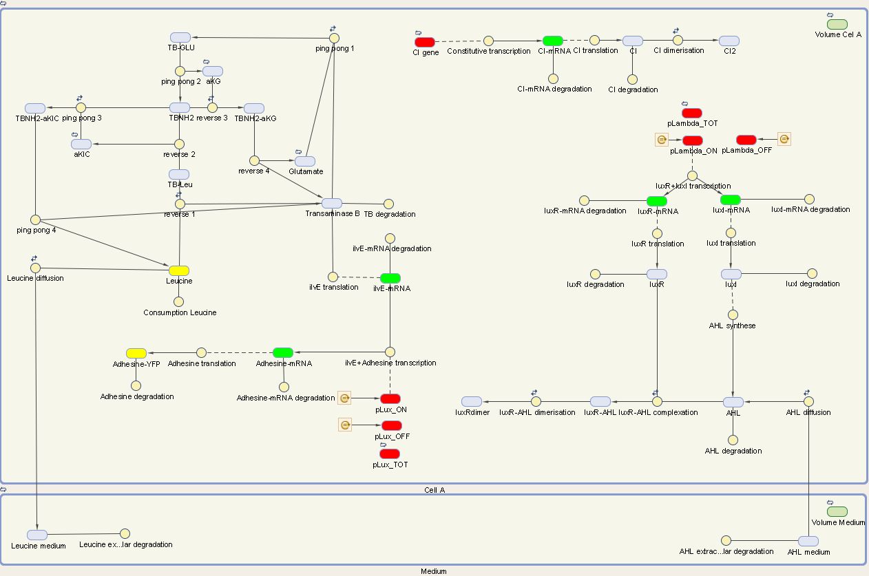
Figure 1: The internal network of cell A visualized by Simbiology
Cell B
The system of cell B is also under control of the cI repressor and is activated similar as cell A. The activation by the temperature raise, leads to the production of LuxR. AHL of the medium can diffuse into the cell, binding LuxR and activating the next component of the circuit. This leads to the production of CheZ and PenI. CheZ is the protein responsible for cells to make a directed movement, governed by the repellent leucine. PenI is a repressor which will shut down the last part of the circuit which was responsible for the production of RFP.
We can extract the following ODEs for cell B from this sytem:
Cell B equations
Symbols: ${\alpha}$:transcription term, ${\beta}$:translation term, $d$:degradation term,
$D$:diffusion term, ${ K_d}$:dissociation constant, n:Hill coefficient, L:leak term
$$\frac{{\large d} m_{cI}}{d t} = \alpha_1 {\cdot} cI_{gene} - d_1 {\cdot} m_{cI}$$ $$\frac{{\large d}{cI}}{d t} = \beta_1 {\cdot} {cI} -2 {\cdot} {k_{cI,dim}} {\cdot} {cI}^2 + 2 {\cdot}{k_{-cI,dim}}{\cdot} {[cI]_2} - d_{cI} {\cdot} {cI} $$
We visualize these ODE's in the Simbiology toolbox. This gives us the following diagrams:
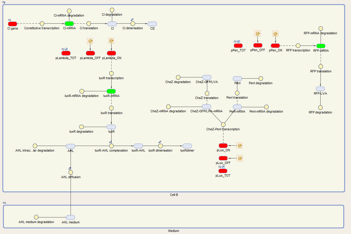
Figure 2: The internal network of cell A visualized by Simbiology
Results
The simulations will be made using ode15s, a solver for stiff systems. We also need to define initial values. We take for the external volume $5{\cdot}10^{-18}l$ as initial value, and for cI-mRNA, cI and $cI_2$ 300,2000, $6{\cdot}10^5$ molecules respectively.
For cell A we made a simulation with cell A in the ON and OFF mode as visuable in figure 3. When cell A is in the OFF state, the whole designed circuit is in OFF mode. This means that the cI repressor is succesful in repressing the design. If the degradation rate of cI is raised to simulate the temperature rising, we see that all the components of the system show a big increase. For LuxR this increase is only temporary, but this is also explainable. Since LuxI keeps on producing AHL which binds LuxR to form a complex. Indeed all the LuxR reacts to form the complex. Some values seem really high (for example the AHL,out en leucine,extracellular values, but they are also in the biggest volume so the concentration is not that high). We also assumed that there is a substrate pool without limiting, which is of course not the real situation. The most important conclusion is that with values backed up by literature, our system qualitatively still shows the desired behavior. We can also ignore noise effects because our model works with a big amount of transcription factors, so small changes will only have a limited effect.
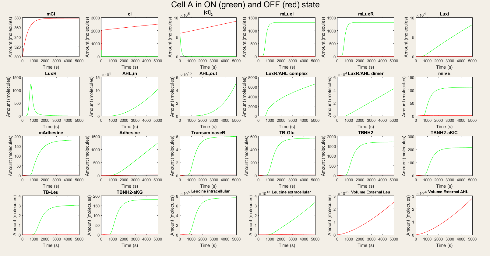
Figure 3: Simulation of all processes in Cell A in ON and OFF state
Afterwards, we made the simulations for cell B. In the OFF state simulations, there is not a big difference between the red and green lines. We do see a very small rise in LuxR but it is not significant. We see a fast equilibration between the external AHL and internal AHL and no drop since there is no LuxR to react with the AHL. The only proteins that are available in high amounts are PenI and RFP. The high amount of PenI was not predicted in our design, but it does not affect the amount of RFP.
In the ON simulations we see a big difference between the red and green lines. When there is AHL available, the production of CheZ and PenI is much higher and the production of RFP much lower. This is expected the behavior. Therefore we conclude that our system is still qualitatively showing the desired behavior.
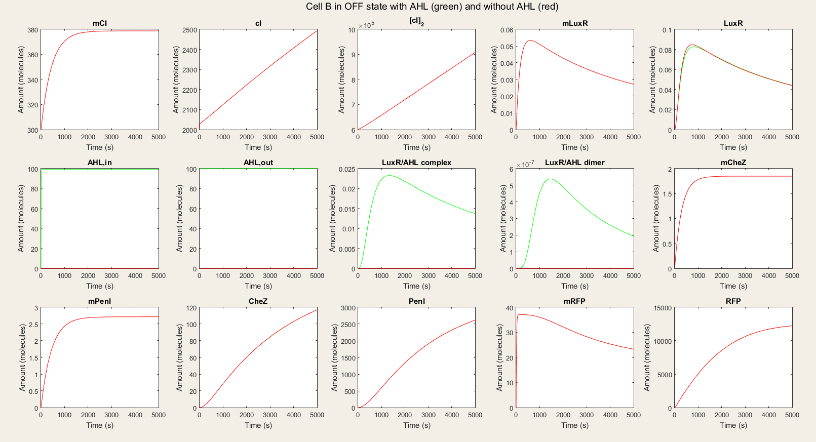
Figure 4: Simulation of all processes in Cell B in OFF state with and without AHL induction
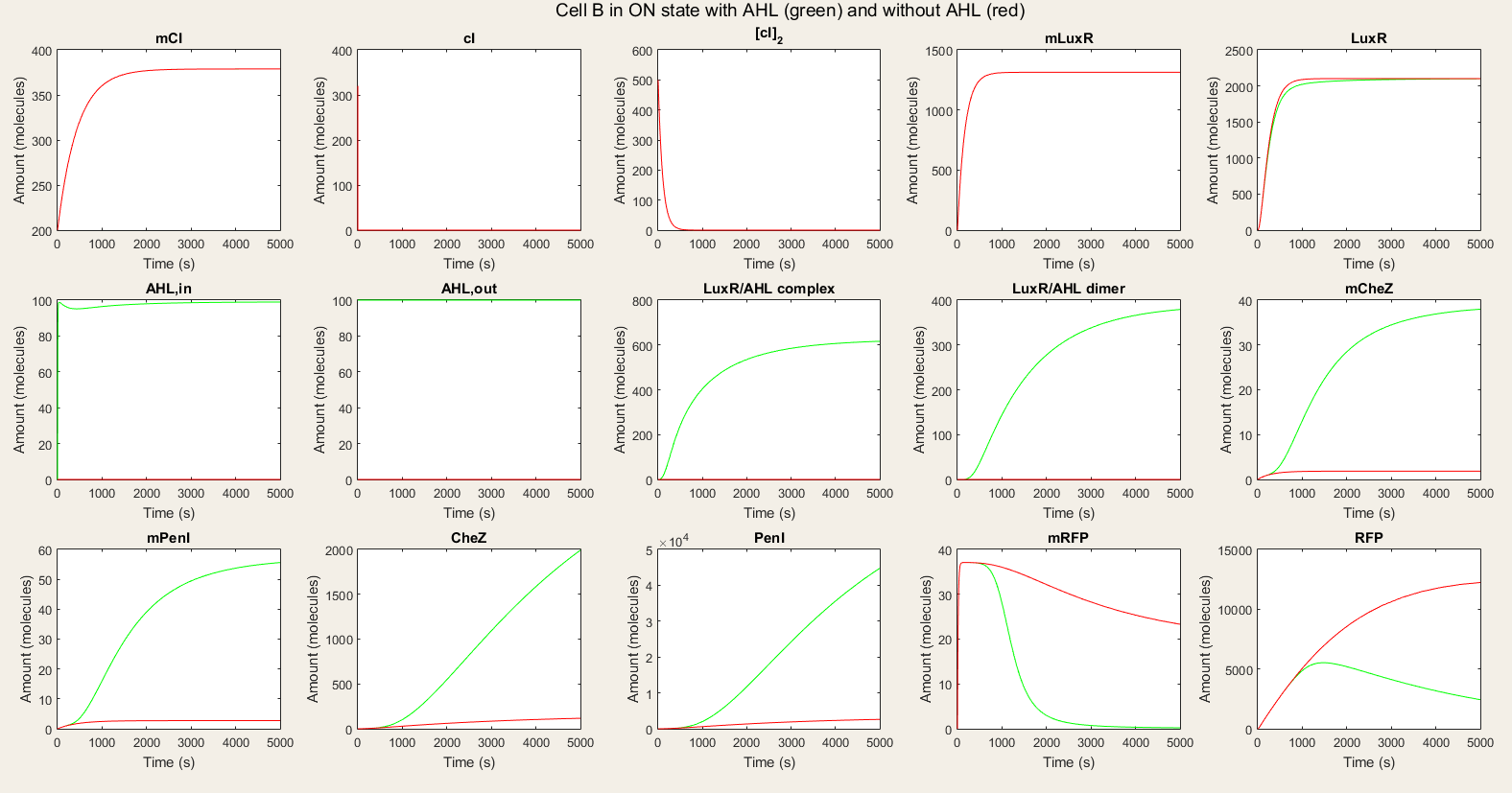
Figure 5: Simulation of all processes in Cell B in ON state with and without AHL induction
It is also important to study the effect of change of AHL on cell B. Thus, we gave cell B a shot of AHL which is degraded in time and watched how it responded on it. Our simulation results were plotted in figure 6. We see that cell B starts with CheZ production untill a maximum, after which production slows down and the protein is degraded. This corresponds with a decrease in AHL concentration. After some time, cell B's internal network has switched and RFP production starts. We notice that the production rate is slower than CheZ production. From this simulation we can conclude that the network we modeled is able to adapt to the AHL concentration and that the reaction is the wanted reaction. We do also notice that it takes a long time (10 000 s) until most CheZ is degraded. This can form a barrier on the real life performance, since only a small amount of CheZ could suffice to give the cells the possibility to move.
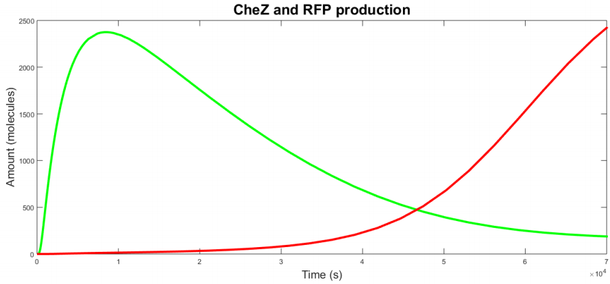
Figure 6: Simulation of cell B with an initial shot of AHL
Sensitivity analysis
Now we are going to check which parameters have the biggest effect on the output and are the most important. We can quantify this effect using derivatives: $\frac{\delta {output}}{\delta {parameter}}$. The parameters with the largest sensitivity values, are the ones that should be best characterized. Furthermore, if they are controllable, they could be varied to our wishes. The sensitivity analysis will be executed in Simbiology. This analysis uses complex-step approximation to calculate derivatives of reaction rates. This technique yields accurate results for the vast majority of typical reaction kinetics including ours. We will use full dedimensionalization so we can compare the results.
For cell A the outputs are the amount of leucine and AHL in the medium and Adhesine. We took a time integral of the sensitivities and plotted it in figure 7.
The leucine medium is dependent on diffusion of leucine out, leucine consumption, degradation, transcription and translation of ilvE mRNA. We also notice that not all Ping-Pong Bi-Bi constants are equally important. The parameters kf1, kf-1 and kcat are the most important while kr1, kr-1 and kcat3 are the least important.
AHL medium is highly sensitive for variations in luxI translation, degradation of LuxI and LuxI mRNA and for the catalytic activity of LuxI.
Adhesine-YFP is sensitive for translation, degradation and transcription.
From these results we can conclude that all outputs are dependent on variables closely related to themselves. Indeed, since there is production of AHL and LuxR in the cell, the transcriptional network is always active so the steps concerning the transcriptional network lose their importance. It is thus only a matter of understanding the metabolism, production and degradation terms to correctly model cell A.
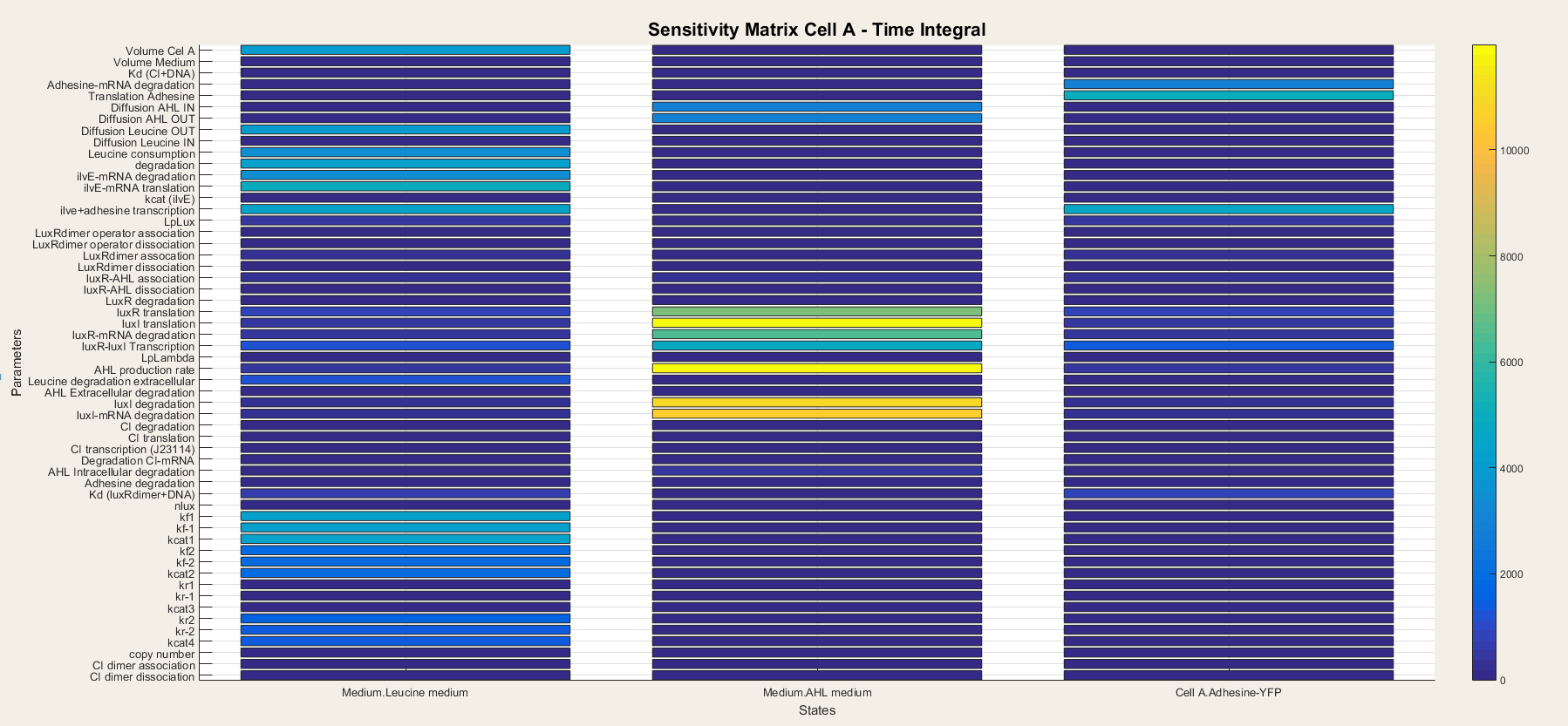
Figure 7: Sensitivity analysis of parameters in cell A
We do the same for cell B. In cell B the output is the production of CheZ and RFP and the results are plotted in figure 8. We notice that CheZ-GFP is highly sensitive for the association rates of the LuxR/AHL complex and the LuxR/AHL dimer. RFP production is also sensitive for the association of the LuxR/AHL dimer.
We see that in cell B the dimerisation steps are really important. This is logical since cell B is dependent on external AHL concentrations to boot the transcriptional network. Thus, the steps concerning the binding of AHL to LuxR and making the activated LuxR/AHL dimer, which starts the transcription, are the most important steps. They determine the sensitivity of the network to AHL and as so, form the major component of the network.
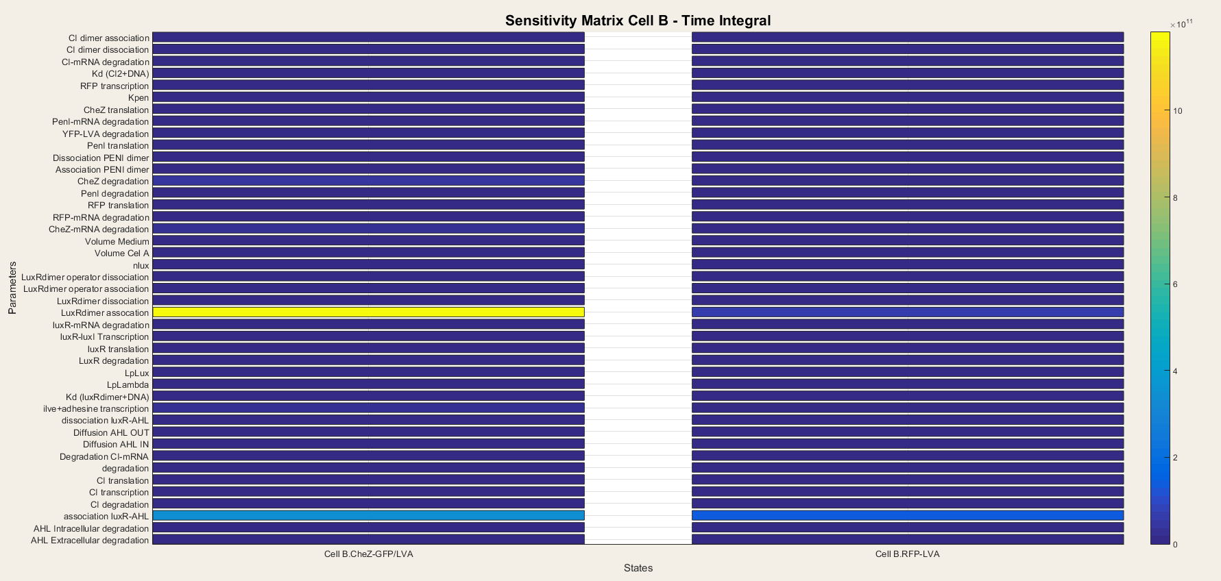
Figure 8: Sensitivity analysis of parameters in cell B
Conclusion
We conclude from these results that our model displays the desired behavior. In both cell A and cell B, there is a big difference between cells in ON and OFF mode. In addition, the presence of AHL also has a big effect on cell B. The simulation also show a problem: altough we equiped the proteins with a LVA-tag, the degradation rate is still very slow and this can affect the cell behavior. We can also get semi-quantitative results from this model, but our assumption of an unlimited substrate pool leads to very high amount of biomolecules. A next step would be to fit some model parameters to wet lab data.
From the sensitivy analysis, we know which parameters are the most important and should be optimized. For cell A we should focus on metabolic, transcriptional and translational terms and for cell B we should focus on the dimerization steps.
References
| [1] | R. P. Shetty and B. Canton. PoPS. Openwetware 2007. [Available at url ] |
| [2] | Jason R Kelly, Adam J Rubin, Joseph H Davis, Caroline M Ajo-Franklin, John Cumbers, Michael J Czar, Kim de Mora, Aaron L Glieberman, Dileep D Monie, and Drew Endy. Measuring the activity of BioBrick promoters using an in vivo reference standard. Journal of biological engineering, 3:4, 2009. [ DOI ] |
| [3] | J N Weiss. The Hill equation revisited: uses and misuses. The FASEB journal : official publication of the Federation of American Societies for Experimental Biology, 11(11):835-841, 1997. [ DOI ] |
| [4] | Yufang Wang, Ling Guo, Ido Golding, Edward C Cox, and N P Ong. Quantitative transcription factor binding kinetics at the single-molecule level. Biophysical Journal, 96(2):609-620, 2009. [ DOI | arXiv | http ] |
| [5] | S. Basu, Y. Gerchman, C.H. Collins, F.H. Arnold and R. Weiss. A synthetic multicellular system for programmed pattern formation. Nature, 434(7037):1130-1134, 2005. [ DOI | |
| [6] | V Wittman, H C Lin, and H C Wong. Functional domains of the penicillinase repressor of Bacillus licheniformis. Journal of Bacteriology, 175(22):7383-7390, 1993. |
| [7] | Farasat I., Kushwaha M., Collens J., Easterbrook M. and H.M. Salis Efficient search, mapping, and optimization of multi-protein genetic systems in diverse bacteria. Molecular systems biology10(6):731, 1998. [ DOI ] |
| [8] | Benjamin Reeve, Thomas Hargest, Charlie Gilbert, and Tom Ellis. Predicting Translation Initiation Rates for Designing Synthetic Biology. Frontiers in Bioengineering and Biotechnology, 2(January):1-6, 2014. [ DOI | http ] |
| [9] | Howard M. Salis, Amin E. Borujeni and Anirudh S. Channarasappa. Translation rate is controlled by coupled trade-offs between site accessibility, selective RNA unfolding and sliding at upstream standby sites. Nucleic Acids Research 42 (2): 2646-2659, 2014. [ DOI | |
| [10] | A. B. Goryachev, D. J. Toh, and T. Lee. Systems analysis of a quorum sensing network: Design constraints imposed by the functional requirements, network topology and kinetic constants. In BioSystems, volume 83, pages 178-187, 2006. [ DOI ] |
| [11] | K T Samiee, M Foquet, L Guo, E C Cox, and H G Craighead. lambda-Repressor oligomerization kinetics at high concentrations using fluorescence correlation spectroscopy in zero-mode waveguides. Biophysical journal, 88(3):2145-2153, 2005. [ DOI | http ] |
| [12] | A L Schaefer, D L Val, B L Hanzelka, J E Cronan, and E P Greenberg. Generation of cell-to-cell signals in quorum sensing: acyl homoserine lactone synthase activity of a purified Vibrio fischeri LuxI protein. Proceedings of the National Academy of Sciences of the United States of America, 93(18):9505-9509, 1996. [ DOI ] |
| [13] | Chin-Rang Yang, Bruce E Shapiro, She-Pin Hung, Eric D Mjolsness, and G Wesley Hatfield. A mathematical model for the branched chain amino acid biosynthetic pathways of Escherichia coli K12. The Journal of biological chemistry, 280(12):11224-11232, 2005. [ DOI ] |
| [14] | Chin Rang Yang, Bruce E Shapiro, Eric D Mjolsness, and G Wesley Hatfield. An enzyme mechanism language for the mathematical modeling of metabolic pathways. Bioinformatics, 21(6):774-780, 2005. [ DOI ] |
| [15] | Jonathan a Bernstein, Arkady B Khodursky, Pei-Hsun Lin, Sue Lin-Chao, and Stanley N Cohen. Global analysis of mRNA decay and abundance in Escherichia coli at single-gene resolution using two-color fluorescent DNA microarrays. Proceedings of the National Academy of Sciences of the United States of America, 99(15):9697-9702, 2002. [ DOI ] |
| [16] | Jens Bo Andersen, Claus Sternberg, Lars Kongsbak Poulsen, Sara Petersen Bjø rn, Michael Givskov, and Sø ren Molin. New unstable variants of green fluorescent protein for studies of transient gene expression in bacteria. Applied and Environmental Microbiology, 64(6):2240-2246, 1998. [ arXiv ] |
| [17] | Horswill A.R., Stoodley P., Stewart P.S. and Parsek M.R. The effect of the chemical, biological, and physical environment on quorum sensing in structured microbial communities Anal Bioanal Chem.387(2):371-380. |


Contact
Address: Celestijnenlaan 200G room 00.08 - 3001 Heverlee
Telephone: +32(0)16 32 73 19
Email: igem@chem.kuleuven.be


