Difference between revisions of "Team:KU Leuven/Modeling/Internal"
| Line 89: | Line 89: | ||
<p> We can think of many relevant questions in implementing a new circuit: how sensitive is the system, how much will it produce and will it affect the growth? As such, it is important to model the effect of the new circuits on the bacteria. This will be done in the Internal Model. We will use two approaches. First we will use a bottom-up approach. This involves building a detailed kinetic model with rate laws. We will use Simbiology and ODE's to study the sensitivity and dynamic processes inside the cell. This is the bottom-up approach. Afterwards, a top-down model, Flux Balance Analysis (FBA), will be used to study the steady-state values for production flux and growth rate. This part is executed by the iGEM Team of Toulouse as part of a collaboration and can be found <a href="https://2015.igem.org/Team:KU_Leuven/Modeling/Toulouse" > here </a> | <p> We can think of many relevant questions in implementing a new circuit: how sensitive is the system, how much will it produce and will it affect the growth? As such, it is important to model the effect of the new circuits on the bacteria. This will be done in the Internal Model. We will use two approaches. First we will use a bottom-up approach. This involves building a detailed kinetic model with rate laws. We will use Simbiology and ODE's to study the sensitivity and dynamic processes inside the cell. This is the bottom-up approach. Afterwards, a top-down model, Flux Balance Analysis (FBA), will be used to study the steady-state values for production flux and growth rate. This part is executed by the iGEM Team of Toulouse as part of a collaboration and can be found <a href="https://2015.igem.org/Team:KU_Leuven/Modeling/Toulouse" > here </a> | ||
</p> | </p> | ||
| − | < | + | </div> |
| − | < | + | <div class="part"> |
<h2> 2. Simbiology and ODE </h2> | <h2> 2. Simbiology and ODE </h2> | ||
<p> | <p> | ||
In the next section we will describe our Simbiology model. Simbiology allows us to calculate systems of ODE's and to visualize the system in a diagram. It also has options to make scans for different parameters, which allows us to study the effect of the specified parameter. We will focus on the production of leucine, Ag43 and AHL in cell A and the changing behavior of cell B due to changing AHL concentration. In this perspective, we will make two models in Simbiology: one for cell A and cell B. First we will describe how we made the model and searched for the parameters. Afterwards we check the robustness of the model with a parameter analysis and we do scans to check for the effects of molecular noise. | In the next section we will describe our Simbiology model. Simbiology allows us to calculate systems of ODE's and to visualize the system in a diagram. It also has options to make scans for different parameters, which allows us to study the effect of the specified parameter. We will focus on the production of leucine, Ag43 and AHL in cell A and the changing behavior of cell B due to changing AHL concentration. In this perspective, we will make two models in Simbiology: one for cell A and cell B. First we will describe how we made the model and searched for the parameters. Afterwards we check the robustness of the model with a parameter analysis and we do scans to check for the effects of molecular noise. | ||
</p> | </p> | ||
| − | < | + | </div> |
| − | < | + | <div class="part"> |
<h2> 3. Quest for parameters </h2> <a name="Transcription"></a> | <h2> 3. Quest for parameters </h2> <a name="Transcription"></a> | ||
<p> | <p> | ||
| Line 107: | Line 107: | ||
</ol> | </ol> | ||
</p> | </p> | ||
| − | < | + | </div> |
| + | </div> | ||
| + | <div class="center"> | ||
| + | <div class="togglebar"> | ||
| + | <div class="toggleone"> | ||
<h3> 3.1 Transcription </h3> <a name="Translation"></a> | <h3> 3.1 Transcription </h3> <a name="Translation"></a> | ||
| + | </div> | ||
| + | <div id="toggleone"> | ||
<p> | <p> | ||
Transcription is the first step of gene expression. It involves the binding of RNA polymerase to the promoter region and the formation of mRNA. The transcription rate is dependent on a number of conditions like the promoter strength and the used strain. Our system has both constitutive promoters, which are always active, and inducable promoters, which can be activated or repressed. <br> </p> | Transcription is the first step of gene expression. It involves the binding of RNA polymerase to the promoter region and the formation of mRNA. The transcription rate is dependent on a number of conditions like the promoter strength and the used strain. Our system has both constitutive promoters, which are always active, and inducable promoters, which can be activated or repressed. <br> </p> | ||
<br> | <br> | ||
| − | + | ||
| − | + | ||
| − | + | ||
| − | + | ||
<b> Maximum Transcription rate </b> <br> <p> | <b> Maximum Transcription rate </b> <br> <p> | ||
<br> | <br> | ||
| Line 184: | Line 187: | ||
<br> | <br> | ||
</div> | </div> | ||
| − | < | + | </div> |
| + | |||
| + | <div class="togglebar"> | ||
| + | <div class="toggletwo"> | ||
| + | |||
<h3> 3.2 Translation </h3> | <h3> 3.2 Translation </h3> | ||
| + | </div> | ||
| + | <div id="toggletwo" > | ||
<p> | <p> | ||
The next step in gene expression is the translation of the synthesized mRNA to a protein. This involves the binding of a ribosome complex to the RBS site of the mRNA, elongation and termination. The initiation step is the rate-limiting step of the three. The translation rate is thus tied to the thermodynamics of RBS-ribosome interaction but other sequences (5’-UTR, Shine-Delgarno,repeats, internal startcodons) and possible secondary structures (hairpins) also play a role (Chiam Yu Ng, Salis). (Fong) Salis et al have developed an algorithm to predict the translation initiation rate based upon thermodynamic calculations. This algorithm is used in the Ribosome Binding Site Calculator (https://salislab.net/software/ , Borujeni & Salis). We used this Calculator to predict the translation rates of our mRNAs. | The next step in gene expression is the translation of the synthesized mRNA to a protein. This involves the binding of a ribosome complex to the RBS site of the mRNA, elongation and termination. The initiation step is the rate-limiting step of the three. The translation rate is thus tied to the thermodynamics of RBS-ribosome interaction but other sequences (5’-UTR, Shine-Delgarno,repeats, internal startcodons) and possible secondary structures (hairpins) also play a role (Chiam Yu Ng, Salis). (Fong) Salis et al have developed an algorithm to predict the translation initiation rate based upon thermodynamic calculations. This algorithm is used in the Ribosome Binding Site Calculator (https://salislab.net/software/ , Borujeni & Salis). We used this Calculator to predict the translation rates of our mRNAs. | ||
</p> | </p> | ||
<br> | <br> | ||
| − | + | ||
| − | + | ||
| − | + | ||
| − | + | ||
<p> | <p> | ||
The results are in table 1. The program gives us results in au (arbitrary units). Since we know the translation rate of LuxI and LuxR, we can use these as a base to calculate the other translation rates since the used scale is proportional. (table 1, column 2) LuxI and LuxR have almost the same output from the calculator which corresponds with the paper where they also have the same translation rate. (Ag43 has a very low translation rate, which is not completely illogical, since Ag43 is by far the biggest protein.) Our values are normal values since 1000 is a moderate value and values between 1 and 100 000 are possible. (efficient search, mapping and optimization, salis). We did get warnings about the prediction (NEQ: not at equilibrium) which happens when mRNA may not fold quickly to its equilibrium state. </p> | The results are in table 1. The program gives us results in au (arbitrary units). Since we know the translation rate of LuxI and LuxR, we can use these as a base to calculate the other translation rates since the used scale is proportional. (table 1, column 2) LuxI and LuxR have almost the same output from the calculator which corresponds with the paper where they also have the same translation rate. (Ag43 has a very low translation rate, which is not completely illogical, since Ag43 is by far the biggest protein.) Our values are normal values since 1000 is a moderate value and values between 1 and 100 000 are possible. (efficient search, mapping and optimization, salis). We did get warnings about the prediction (NEQ: not at equilibrium) which happens when mRNA may not fold quickly to its equilibrium state. </p> | ||
| Line 247: | Line 253: | ||
</div> | </div> | ||
| − | + | </div> | |
| − | + | ||
| + | <div class="togglebar"> | ||
| + | <div class="togglethree"> | ||
<h3> 3.3 Complexation and dimerization </h3> | <h3> 3.3 Complexation and dimerization </h3> | ||
| + | </div> | ||
| + | <div id="togglethree" > | ||
<p> | <p> | ||
Before the proteins can bind the promoter region, they first have to make complexes. cI and penI form homodimers, while LuxR first forms a heterodimer with AHL and afterwards forms a homodimer with another LuxR/AHL dimer. This next part will describe the kinetics of such complexation. We only need the parameters of LuxR and cI, because the Hill function found for penI already was adapted for the protein in monomer form. <br> | Before the proteins can bind the promoter region, they first have to make complexes. cI and penI form homodimers, while LuxR first forms a heterodimer with AHL and afterwards forms a homodimer with another LuxR/AHL dimer. This next part will describe the kinetics of such complexation. We only need the parameters of LuxR and cI, because the Hill function found for penI already was adapted for the protein in monomer form. <br> | ||
| − | <br> | + | <br></p> |
<div class="datatable"> | <div class="datatable"> | ||
<table> | <table> | ||
| Line 293: | Line 302: | ||
</table> | </table> | ||
</div> | </div> | ||
| − | </ | + | |
| + | </div> | ||
| + | </div> | ||
| + | |||
| + | <div class="togglebar"> | ||
| + | <div class="togglefour"> | ||
<h3> 3.4 Protein production kinetics </h3> | <h3> 3.4 Protein production kinetics </h3> | ||
| + | </div> | ||
| + | <div id="togglefour"> | ||
<p>Our models comprise two product forming enzymes: LuxI and Transaminase B. | <p>Our models comprise two product forming enzymes: LuxI and Transaminase B. | ||
LuxI is the enzyme responsible for AHL production and Transaminase B is responsible for Leucine formation. <br> | LuxI is the enzyme responsible for AHL production and Transaminase B is responsible for Leucine formation. <br> | ||
| Line 377: | Line 393: | ||
</div> | </div> | ||
| + | </div> | ||
| + | </div> | ||
| + | |||
| + | <div class="togglebar"> | ||
| + | <div class="togglefive"> | ||
<h3> 3.5 Degradation </h3> | <h3> 3.5 Degradation </h3> | ||
| + | </div> | ||
| + | <div id="togglefive"> | ||
| + | |||
<p>Proteins, mRNA and other metabolites have a turnover rate. They are degraded over time. The degradation rate will be described as proportional to the amount of biomolecules. The coefficient of proportionality d is the degradation constant. Not every molecule has the same degradation rate, since some molecules are more stable than others. We can influence the stability of the molecules. For example, in cell B it is important that there is a fast switch between conditions and a fast turnover of CheZ and RFP is necessary. This is why we add a LVA-tag to these proteins. This tag destabilizes the protein and makes them degradade faster. For TransaminaseB we choose a very high degradation rate, because we did not include degradation terms for the TransaminaseB bound to substrate. The degradation rates used in the model are put in the next table: <p> | <p>Proteins, mRNA and other metabolites have a turnover rate. They are degraded over time. The degradation rate will be described as proportional to the amount of biomolecules. The coefficient of proportionality d is the degradation constant. Not every molecule has the same degradation rate, since some molecules are more stable than others. We can influence the stability of the molecules. For example, in cell B it is important that there is a fast switch between conditions and a fast turnover of CheZ and RFP is necessary. This is why we add a LVA-tag to these proteins. This tag destabilizes the protein and makes them degradade faster. For TransaminaseB we choose a very high degradation rate, because we did not include degradation terms for the TransaminaseB bound to substrate. The degradation rates used in the model are put in the next table: <p> | ||
<div class="datatable"> | <div class="datatable"> | ||
| Line 489: | Line 513: | ||
</div> | </div> | ||
| + | </div> | ||
| + | </div> | ||
| + | |||
| + | <div class="togglebar"> | ||
| + | <div class="togglesix"> | ||
<h3> 3.6 Diffusion </h3> | <h3> 3.6 Diffusion </h3> | ||
| + | </div> | ||
| + | </div> | ||
| + | <div id="togglesix"> | ||
<p> | <p> | ||
Our model has 2 types of diffusion. Diffusion from the inside of the cell to the outside over the cell membrane and diffusion in the external medium. The diffusion over the cell membrane is more complicated because some proteins play a role in it and the membrane is not equally permeable for every molecule. For AHL, we found a value given in molecules/second. This unit seems strange because diffusion is usually used with units in concentration. It also leads to strange results since the amount of molecules is being leveled out so the inside amount equals the outside amount even though the concentrations are different. This is why we added a correction for the volume of the cell and the external volume to it. <br> </p> | Our model has 2 types of diffusion. Diffusion from the inside of the cell to the outside over the cell membrane and diffusion in the external medium. The diffusion over the cell membrane is more complicated because some proteins play a role in it and the membrane is not equally permeable for every molecule. For AHL, we found a value given in molecules/second. This unit seems strange because diffusion is usually used with units in concentration. It also leads to strange results since the amount of molecules is being leveled out so the inside amount equals the outside amount even though the concentrations are different. This is why we added a correction for the volume of the cell and the external volume to it. <br> </p> | ||
<br> | <br> | ||
| − | |||
| − | |||
| − | |||
| − | |||
<br> | <br> | ||
<p> | <p> | ||
| Line 539: | Line 567: | ||
</div> | </div> | ||
</div> | </div> | ||
| − | < | + | </div> |
| + | </div> | ||
| + | |||
<h3> 4. System </h4><br> | <h3> 4. System </h4><br> | ||
| Line 582: | Line 612: | ||
$$\frac{{\large d}{[{TBNH}_2-aKG]}}{d t}= {kr}_2{\cdot}{{TBNH}_2}{\cdot}{aKG} - {kr}_{2}{\cdot}{[{TBNH}_2-aKG]} - {kcat4}{\cdot}{[{TBNH}_2-aKG]}$$ | $$\frac{{\large d}{[{TBNH}_2-aKG]}}{d t}= {kr}_2{\cdot}{{TBNH}_2}{\cdot}{aKG} - {kr}_{2}{\cdot}{[{TBNH}_2-aKG]} - {kcat4}{\cdot}{[{TBNH}_2-aKG]}$$ | ||
</div> | </div> | ||
| − | + | ||
</p> | </p> | ||
</div> | </div> | ||
| Line 610: | Line 640: | ||
$$\frac{{\large d}{cI}}{d t} = \beta_1 {\cdot} {cI} -2 {\cdot} {k_{cI,dim}} {\cdot} {cI}^2 + 2 {\cdot}{k_{-cI,dim}}{\cdot} {[cI]_2} - d_{cI} {\cdot} {cI} $$ | $$\frac{{\large d}{cI}}{d t} = \beta_1 {\cdot} {cI} -2 {\cdot} {k_{cI,dim}} {\cdot} {cI}^2 + 2 {\cdot}{k_{-cI,dim}}{\cdot} {[cI]_2} - d_{cI} {\cdot} {cI} $$ | ||
</p> | </p> | ||
| − | + | ||
| − | + | ||
| − | + | ||
| − | + | ||
<p name="Bhidden" id="Bhidden" > | <p name="Bhidden" id="Bhidden" > | ||
$$\frac{{\large d}{[cI]_2}}{d t}= k_{cI,dim} {\cdot} {cI}^2 - {k_{-cI,dim}}{\cdot} {[cI]_2} $$ | $$\frac{{\large d}{[cI]_2}}{d t}= k_{cI,dim} {\cdot} {cI}^2 - {k_{-cI,dim}}{\cdot} {[cI]_2} $$ | ||
| Line 629: | Line 656: | ||
$$\frac{{\large d} RFP}{d t} = \beta_{RFP} {\cdot}{m_{RFP}} - d_{RFP} {\cdot}{RFP} $$ | $$\frac{{\large d} RFP}{d t} = \beta_{RFP} {\cdot}{m_{RFP}} - d_{RFP} {\cdot}{RFP} $$ | ||
</div> | </div> | ||
| − | |||
</p> | </p> | ||
</p> | </p> | ||
| Line 1,032: | Line 1,058: | ||
</body> | </body> | ||
| + | |||
| + | <script> | ||
| + | $("document").ready(function(){ | ||
| + | $("#toggleone").hide(); | ||
| + | $("#toggletwo").hide(); | ||
| + | $("#togglethree").hide(); | ||
| + | $("#togglefour").hide(); | ||
| + | $("#togglefive").hide(); | ||
| + | $("#togglesix").hide(); | ||
| + | $("#toggleseven").hide(); | ||
| + | $("#toggleeight").hide(); | ||
| + | $("#togglenine").hide(); | ||
| + | |||
| + | |||
| + | }); | ||
| + | |||
| + | </script> | ||
| + | <script> | ||
| + | $(".toggleone").click(function () { | ||
| + | $("#toggleone").toggle(); | ||
| + | }); | ||
| + | $(".toggletwo").click(function () { | ||
| + | $("#toggletwo").toggle(); | ||
| + | }); | ||
| + | $(".togglethree").click(function () { | ||
| + | $("#togglethree").toggle(); | ||
| + | }); | ||
| + | $(".togglefour").click(function () { | ||
| + | $("#togglefour").toggle(); | ||
| + | }); | ||
| + | $(".togglefive").click(function () { | ||
| + | $("#togglefive").toggle(); | ||
| + | }); | ||
| + | $(".togglesix").click(function () { | ||
| + | $("#togglesix").toggle(); | ||
| + | }); | ||
| + | $(".toggleseven").click(function () { | ||
| + | $("#toggleseven").toggle(); | ||
| + | }); | ||
| + | $(".toggleeight").click(function () { | ||
| + | $("#toggleeight").toggle(); | ||
| + | }); | ||
| + | $(".togglenine").click(function () { | ||
| + | $("#togglenine").toggle(); | ||
| + | }); | ||
| + | </script> | ||
</html> | </html> | ||
Revision as of 21:47, 16 September 2015

Internal Model
1. Introduction
We can think of many relevant questions in implementing a new circuit: how sensitive is the system, how much will it produce and will it affect the growth? As such, it is important to model the effect of the new circuits on the bacteria. This will be done in the Internal Model. We will use two approaches. First we will use a bottom-up approach. This involves building a detailed kinetic model with rate laws. We will use Simbiology and ODE's to study the sensitivity and dynamic processes inside the cell. This is the bottom-up approach. Afterwards, a top-down model, Flux Balance Analysis (FBA), will be used to study the steady-state values for production flux and growth rate. This part is executed by the iGEM Team of Toulouse as part of a collaboration and can be found here
2. Simbiology and ODE
In the next section we will describe our Simbiology model. Simbiology allows us to calculate systems of ODE's and to visualize the system in a diagram. It also has options to make scans for different parameters, which allows us to study the effect of the specified parameter. We will focus on the production of leucine, Ag43 and AHL in cell A and the changing behavior of cell B due to changing AHL concentration. In this perspective, we will make two models in Simbiology: one for cell A and cell B. First we will describe how we made the model and searched for the parameters. Afterwards we check the robustness of the model with a parameter analysis and we do scans to check for the effects of molecular noise.
3. Quest for parameters
We can divide the different processes that are being executed in the cells in 7 classes: transcription, translation, DNA binding, complexation and dimerization, protein production kinetics, degradation and diffusion. We went on to search the necessary parameters and descriptions for each of these categories. To start making our model we have to chose a unit. We choose to use molecules as unit because many constants are expressed in this unit and it allows us to drop the dillution terms connected to cell growth. We will also work with a deterministic model instead of a stochastic model. A stochastic model will show us the molecular noise, but we will check this with parameter scans.
The next step is to make some assumptions:
- The effects of cell division can be neglected
- The substrate pool can not be depleted and the concentration (or amount of molecules) of substrate in the cell is constant
- The exterior of the cell contains no leucine at t=0 and is perfectly mixed
- Diffusion happens independent of cell movement and has a constant rate
Our model has 2 types of diffusion. Diffusion from the inside of the cell to the outside over the cell membrane and diffusion in the external medium. The diffusion over the cell membrane is more complicated because some proteins play a role in it and the membrane is not equally permeable for every molecule. For AHL, we found a value given in molecules/second. This unit seems strange because diffusion is usually used with units in concentration. It also leads to strange results since the amount of molecules is being leveled out so the inside amount equals the outside amount even though the concentrations are different. This is why we added a correction for the volume of the cell and the external volume to it.
We assume that the volume of the cell has a shape of a cilinder and is constant. For this simplified volume we found a value of $5.65 {\cdot} 10^{-16} $ l. We can take this volume as a constant, since cell growth is very small compared to the diffusion. The outside compartment will be modeled as half a sphere with the cell as center and a radius equal to $\sqrt{2*D*t}$ + r0. We only take half a sphere because there is no upward diffusion. For the initial value of the outside compartment we take a volume (and thus r0 slightly bigger than the cell volume (radius).
With this approximation we get more logical results. We take the diffusion rate for AHL equal to 0.23 1/s. For Leucine we make a differce between inward and outward diffusion. Inward diffusion is facilitated by transporters, so we choose this value to be the largest. The inward diffusion rate is
| Biomolecule | Diffusion rate (1/s) | Source |
|---|---|---|
| AHL IN and OUT | 0.23 1/s | Goryachev et al. (2005) |
| Leucine IN | 0.05 1/s | Estimated |
| Leucine OUT | 0.0005 1/s | Estimated |
| AHL extracellular | $7.1{\cdot}10^{-9}$ dm²/s | Goryachev et al. (2005) |
| Leucine extracellular | $7.3{\cdot}10^{-8}{\cdot}0.09$ dm²/s | iGEM Aberdeen 2009 |
4. System
4.1 Cell A
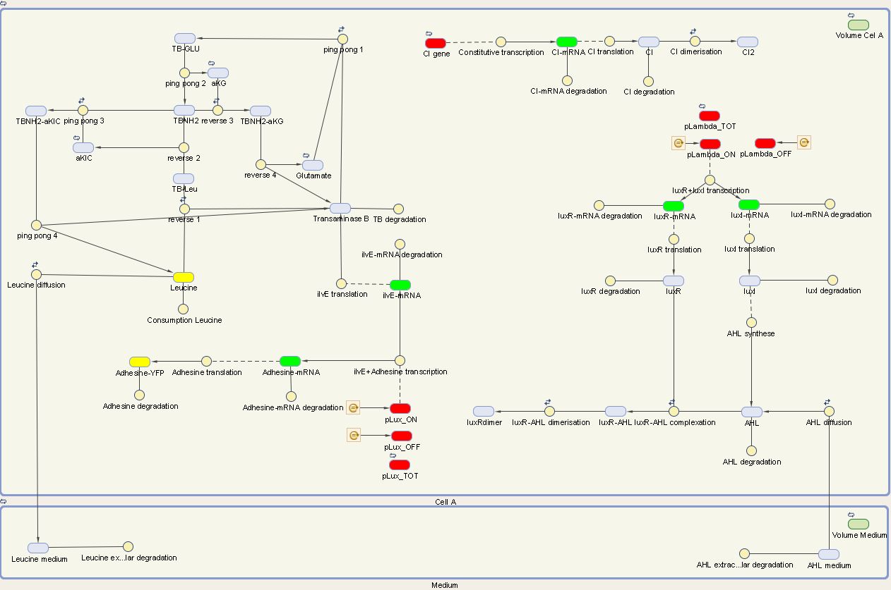
The designed circuit in Cell A is under control of a temperature sensitive cI repressor. Upon raising the temperature, cI will dissociate from the promoter and the circuit is activated. This leads to the initiation of the production of LuxR and LuxI. LuxI will consecutively produce AHL, which binds with LuxR. The newly formed complex will then activate the production of Leucine and Ag43. Leucine and AHL are also able to diffuse out of the cell into the medium. Ag43 is the adhesine which aids the aggregation of cells A, while Leucine and AHL are necessary to repel cells B.
We can extract the following ODE's from this circuit:
Cell A equations
Symbols:${}$ ${\alpha}$: transcription term, ${\beta}$: translation term, $d$: degradation term,
$D$: diffusion term, ${ K_d}$: dissociation constant, n: Hill coefficient, L: leak term
$$\frac{{\large d} m_{cI}}{d t} = \alpha_1 {\cdot} cI_{gene} - d_{mCI} {\cdot} m_{cI}$$ \begin{align} \frac{{\large d}{cI}}{d t} = \beta_{cI} {\cdot} {m_{cI}} -2 {\cdot} {k_{cI,dim}} {\cdot} {cI}^2 + 2 {\cdot} {k_{-cI,dim}}{\cdot} {[cI]_2} - d_{cI} {\cdot} {cI} \end{align}
We visualize these ODE's in the Simbiology Toolbox which results in the following diagram:
4.2 Cell B
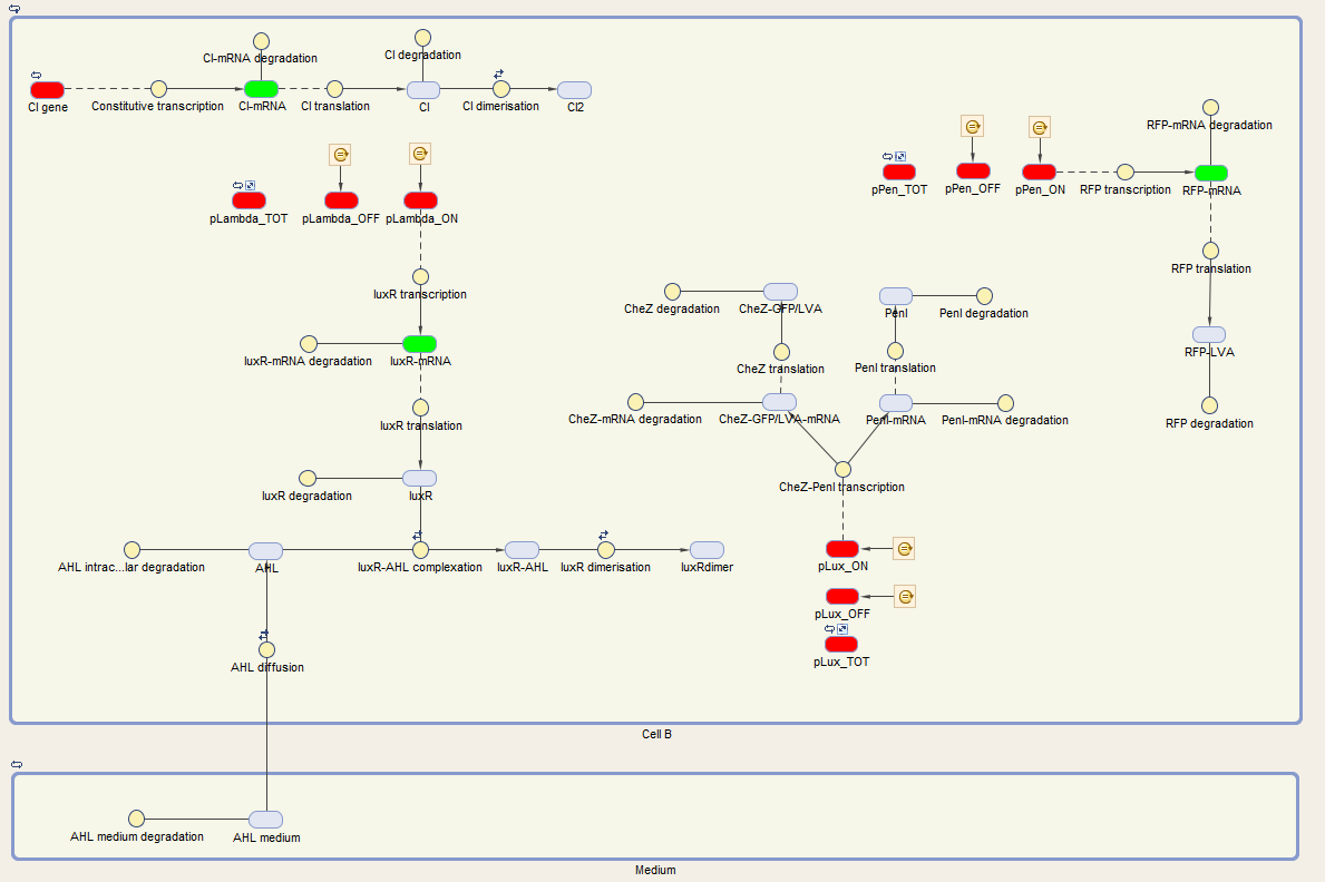
The system of Cell B is also under control of the cI repressor and is activated similar as cell A. The activation by the temperature raise, leads to the production of LuxR. AHL of the medium can diffuse into the cell, binding LuxR and activating the next component of the circuit. This leads to the production of CheZ and PenI. CheZ is the protein responsible for cells to make a directed movement, governed by the repellent Leucine. PenI is a repressor which will shut down the last part of the circuit which was responsible for the production of RFP.
We can extract the following ODEs for Cell B from this sytem:
Cell B equations
Symbols: ${\alpha}$:transcription term, ${\beta}$:translation term, $d$:degradation term,
$D$:diffusion term, ${ K_d}$:dissociation constant, n:Hill coefficient, L:leak term
$$\frac{{\large d} m_{cI}}{d t} = \alpha_1 {\cdot} cI_{gene} - d_1 {\cdot} m_{cI}$$ $$\frac{{\large d}{cI}}{d t} = \beta_1 {\cdot} {cI} -2 {\cdot} {k_{cI,dim}} {\cdot} {cI}^2 + 2 {\cdot}{k_{-cI,dim}}{\cdot} {[cI]_2} - d_{cI} {\cdot} {cI} $$
We visualize these ODE's in the Simbiology toolbox. This gives us the following diagrams:
5. Results
Cell A graph of all, graph of Leucine, graph of AHL
Cell B graph of all, graph with induction and without induction
Sensitivity analysis
Conclusion and discussion


