Difference between revisions of "Team:KU Leuven/Modeling/Hybrid"
| Line 609: | Line 609: | ||
</div> | </div> | ||
<div class="summarytext1"> | <div class="summarytext1"> | ||
| + | <div class="center"> | ||
<div class="togglebar"> | <div class="togglebar"> | ||
<div class="toggleeight"> | <div class="toggleeight"> | ||
Revision as of 22:21, 18 September 2015

The hybrid model
The hybrid model represents an intermediate level of detail in between the colony level model and the internal model. Bacteria are treated as individual agents that behave according to the Keller-Segel type discretized stochastic differential equations, while chemical species are modeled using partial differential equations.
Model Description
Agent-based
To model bacteria movement on the other hand, we used an agent-based model that explicitly stored individual bacteria as agents. Spatial coordinates were associated with each agent, which specified their location. After solving the equation of motion for all agents based on their environment, these coordinates were updated at every timestep. In principle, Newton’s second law of motion had to be solved for all bacteria. However, since bacteria live in a low Reynolds (high friction) environment, the inertia of the bacteria can be neglected. This is because an applied force will immediately be balanced out by an opposing frictional force, with no noticeable acceleration or deceleration phase taking place. $$ \frac{d^2 \vec{r}(t)}{dt^2}=\sum_{i} \vec{F}_{applied,i}-\gamma \cdot \frac{d \vec{r}(t)}{dt}=0 $$ $$\Rightarrow \frac{d \vec{r}(t)}{dt}=\frac{1}{\gamma} \cdot \sum_{i} \vec{F}_{applied,i} \;\;\; \text{(5)} $$ This eliminates the inertial term and simplifies Newton’s second law to (Eq. 5). Basically, the velocity can be calculated as the sum of all applied forces times a constant. For more info about the Reynolds number and “life at low Reynolds number” we refer to box 2.
Stochastic Differential Equation
However, the physical “chemotactic force” that propel bacteria is not easily measured or derived. Therefore, we base the equation of motion in one dimension on (Eq. 6), a stochastic differential equation (SDE) that describes the motion of a single particle in a N-particle system that is governed by a Keller-Segel type PDE in the limit of N → ∞, $$ \frac{\partial n(\vec{r},t)}{\partial t}=D_n \cdot \nabla^2 n - \nabla (n \cdot \chi(S(\vec{r},t)) \cdot\nabla S(\vec{r},t)) \;\;\; (7) $$ more precisely the (Eq. 7) PDE for chemotaxis towards some chemoattractant S. That means that when infinitely many particles obey (Eq. 6), they will exhibit Keller-Segel type spatial dynamics. In a sense, we’re using a “reverse-engineered” particle equation that corresponds to the Keller-Segel field equation. A detailed theoretical treatment of (Eq. 6) is outside the scope of this model description because it contains a stochastic variable. The traditional rules of calculus do not apply anymore for stochastic differential equations and a different mathematical theory called Itō calculus is required. It is sufficient to say that the second term containing dW accounts for Brownian motion in the form of random noise added to the displacement of the agents, causing them to diffuse, and that it is governed by the diffusion coefficient $\mu A$. The first term in (Eq. 6) on the other hand is easily understood as an advective or drift term (net motion) depending on S, pushing the agents along a positive gradient (for negative chemotaxis the sign is reversed). The chemotactic force hence points towards an increasing concentration of the chemoattractant. The advective properties are governed by the chemotactic sensitivity function $\chi (S)$. For our model we defined the chemotactic sensitivity function as in (Eq. 8). $$ \chi(S(\vec{r},t))=\mu \cdot \frac{\kappa}{S(\vec{r},t)} \;\;\; (8) $$ $$ \vec{F}_{cell-cell}=\frac{dE_p(r)}{dr}\cdot\vec{e}_r \;\;\; (9) $$ The first important thing to note is that we assumed $\chi (S)$ to be proportional to 1/S. This is because Keller and Segel proved that their corresponding PDE model only yields travelling wave solutions if $\chi (S)$ contains a singularity at some critical concentration $S_{crit}$, and multiplying by $1/S$ is the simplest way to introduce a singularity at $S_{crit} = 0$. Secondly, the proportionality constant is composed of two factors, namely the bacterial diffusion coefficient $\mu$ and chemotactic sensitivity constant $\kappa$. This is done for two reasons. Firstly, when $\mu$ is lowered, both chemotactic and random motion is reduced, which emulates the state of inactivated motility due to high or low concentrations of AHL. Secondly, defining a separate chemotactic sensitivity constant allows us to examine the effect of the relative strength of chemotaxis versus random motion on pattern formation.
Cell-cell Interactions
In addition to chemotaxis and diffusion, cell-cell interactions play an
important role in pattern formation and also need to be modeled. Bacteria have
finite size and therefore multiple bacteria cannot occupy the same space.
Moreover, an important mechanism in our system is the aggregation of cells A due
to the sticky adhesin protein membrane. To take these mechanisms into account we
modeled two types of cell-cell interactions: the purely repulsive interaction of
cell B with another cell B and with cell A, and the repulsive-attractive
interaction of cell A with another cell A. The interaction between two cells is
usually expressed by a potential energy curve defined over the distance between
the centers of mass of the two cells (fig2). Note that the potential energy
remains constant after a certain distance, which means that the cells stop
interacting. Also, as two cells move closer together, they hit a wall where the
potential energy curve abruptly goes to infinity. The reason for this is that
two cells cannot occupy the same space and therefore smaller intercellular
distances are not allowed. Implementing this theoretical potential is however
not possible because the bacteria are stochastic and could randomly jump beyond
the potential wall, where the force is ill defined. Practically, we’ve decided
to define a piecewise quadratic potential (Eq. 10),
$$ E_{p,attraction}(r_{ij})=\left\{\begin{matrix}
0 & 2\cdot r_{cutoff}\leq r_{ij}\\
-\frac{1}{2}\cdot k_3 \cdot(r_{ij}-2\cdot r_0)^2 & 2\cdot r_0 \leq r_{ij} < 2 \cdot r_{cutoff} \\
-\frac{1}{2}\cdot k_2 \cdot(r_{ij}-2\cdot r_0)^2 & r_0 \leq r_{ij} < 2\cdot r_0\\
-\frac{1}{2}\cdot k_1 \cdot(r_{ij}-\frac{k_1+k_2}{k_1}\cdot r_0)^2 & 0 \leq r_{ij} < r_0
\end{matrix}\right. $$
$$ E_{p,repulsion}(r_{ij})=\left\{\begin{matrix}
0 & 2\cdot r_0\leq r_{ij}\\
-\frac{1}{2}\cdot k_2 \cdot(r_{ij}-2\cdot r_0)^2 & r_0 \leq r_{ij} < 2\cdot r_0\\
-\frac{1}{2}\cdot k_1 \cdot(r_{ij}-\frac{k_1+k_2}{k_1}\cdot r_0)^2 & 0 \leq r_{ij} < r_0
\end{matrix}\right. \;\;\; (10a) $$
$$ \vec{F}_{ij,attraction}(r_{ij})=\left\{\begin{matrix}
\vec{0} & 2\cdot r_{cutoff}\leq r_{ij}\\
k_3 \cdot(r_{ij}-2\cdot r_0) \cdot \vec{e}_{ij} & 2\cdot r_0 \leq r_{ij} < 2 \cdot r_{cutoff} \\
k_2 \cdot(r_{ij}-2\cdot r_0) \cdot \vec{e}_{ij} & r_0 \leq r_{ij} < 2\cdot r_0\\
k_1 \cdot(r_{ij}-\frac{k_1+k_2}{k_1}\cdot r_0) \cdot \vec{e}_{ij} & 0 \leq r_{ij} < r_0
\end{matrix}\right.
$$
$$ \vec{F}_{ij,repulsion}(r_{ij})=\left\{\begin{matrix}
\vec{0} & 2\cdot r_0\leq r_{ij}\\
k_2 \cdot(r_{ij}-2\cdot r_0) \cdot \vec{e}_{ij}& r_0 \leq r_{ij} < 2\cdot r_0\\
k_1 \cdot(r_{ij}-\frac{k_1+k_2}{k_1}\cdot r_0) \cdot \vec{e}_{ij}& 0 \leq r_{ij} < r_0
\end{matrix}\right. \;\;\; (10b)
$$
which results in a piecewise
linear force that resembles Hooke’s law, but with three different “spring
constants” acting in different intervals of intercellular distances (Eq. 10b).
Between A type cells, there is a region of attraction (2*r0 < r < 2*rcutoff),
where the force points towards the other cell, hence moving them closer together.
In the repulsive domain (r < 2*r0), two regions were defined, emulating lower
repulsive forces (r0 < r < 2*r0) and higher repulsive forces due to a higher spring
constant when the cells are even closer (r < r0). For the purely repulsive interaction
scheme there is no attraction and therefore the spring constant for r > 2*r0 is zero.
More details about the implementation of the cell-cell interaction scheme, more specifically
regarding the nearest-neighbor search algorithm, can be found in the paragraph on the agent-based
module below.
Equation of Motion
Now we are ready to construct the equation of motion for cell type A and B as a
superposition of the Keller-Segel SDE (Eq. 6) and the cell interaction forces,
yielding (Eq. 11).
$$ d\vec{r}_{A_i}(t)= \sqrt{2 \cdot \mu_A}\cdot d\vec{W} + \frac{1}{\gamma}\cdot\Bigg( \sum^{A
\backslash \{ A_i\}}_j \frac{dE_{p,attraction}(r_{ij}(t))}{dr_{ij}}\cdot \vec{e}_{ij}+\sum^{B}_j
\frac{dE_{p,repulsion}(r_{ij}(t))}{dr_{ij}}\cdot \vec{e}_{ij} \Bigg)\cdot dt \;\;\; (11a)
$$
$$
d\vec{r}_{B_i}(t)= \chi(L(\vec{r},t),H(\vec{r},t)) \cdot \nabla L(\vec{r},t)\cdot dt + \sqrt{2
\cdot \mu_B(H(\vec{r},t))}\cdot d\vec{W} +
$$
$$
\frac{1}{\gamma}\cdot\Bigg( \sum^{A\cup B\backslash
\{ B_i\}}_j \frac{dE_{p,repulsion}(r_{ij}(t))}{dr_{ij}}\cdot \vec{e}_{ij} \Bigg)\cdot dt
$$
$$
\chi(L(\vec{r},t),H(\vec{r},t))= \mu_{B}(H(\vec{r},t)) \cdot \frac{\kappa}{L(\vec{r},t)}
$$
$$
\mu_A(H(\vec{r},t))=\left\{\begin{matrix}\mu_{A,high} & H(\vec{r},t) < H_{A,threshold}\\
\mu_{A,low} & H(\vec{r},t) \geq H_{A,threshold}\end{matrix}\right.
$$
$$
\mu_B(H(\vec{r},t))=\left\{\begin{matrix}
\mu_{B,high} & H(\vec{r},t) < H_{B,threshold}\\
\mu_{B,low} & H(\vec{r},t) \geq H_{B,threshold}
\end{matrix}\right. \;\;\; \text{(11b)}
$$
Bacteria of type A are not attracted nor repelled by leucine,
so the chemotactic term falls away. All cell-cell forces are summed up to find a
net force, taking into account the two different potentials due to the different
interaction types. As discussed before, this net force times a constant yields
the velocity due to that force, which is then multiplied by dt to obtain the
displacement. For B type cells, the chemotactic term models the repulsive
chemotaxis away from leucine. The chemotactic sensitivity function has a
negative sign signifying that B type cells are repelled by leucine. The cell
interaction term in this case is simpler because B type cells only interact
repulsively. Note that the diffusion coefficient of cell types A and B switches
based on the local concentration of AHL relative to a threshold AHL value, which
simulates the dependency of cellular motility on AHL. The agent-based module is
now fully defined but one crucial issue was skipped: AHL and leucine
concentrations are calculated using PDEs and are therefore only known at grid
points. Agents on the other hand reside in the space between grid points and
require local concentrations as inputs to calculate their next step. This
problem is part of the coupling aspect in our hybrid modelling framework and is
discussed below.
Heat equation
The left-hand side of (1) is the rate of accumulation of a chemical and the right-hand side is the second spatial derivative of its concentration field. The equation can be understood by considering a one-dimensional concentration profile: if (box fig1a) the concentration is higher at both sides of a certain point, it can be approximated as a convex parabolic function. Its second derivative is positive and therefore the rate of accumulation is positive (i.e. more accumulation). If on the other hand (box fig1b) the concentration is lower on both sides of a certain point, a concave function is the correct approximation. The second derivative is therefore negative and the rate of accumulation as well (i.e. depletion). Lastly it is also possible that a lower concentration is found on one side and a higher concentration on the other. In general, the rate of accumulation (accumulation or depletion) depends on the relative differences in concentration between a point and its environment. A special case occurs when the concentration profile takes on a linear form (box fig1c). This means that the differences on both sides of the point are equal in magnitude.
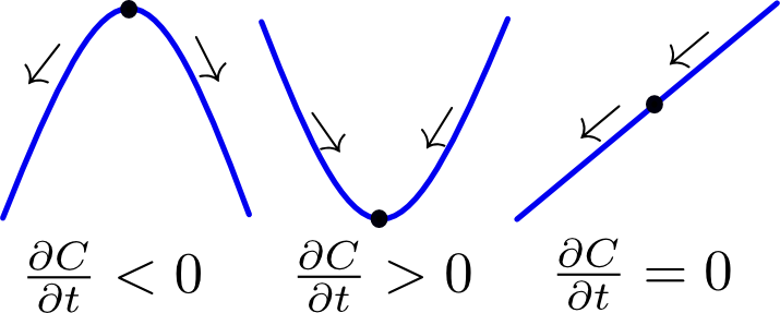
Figure 1 Illustration of the heat euqation. Click to enlarge
Life at low Reynolds number
An important parameter in fluid mechanics is the dimensionless Reynolds number, defined as the ratio of inertial forces to viscous forces, (Eq box 2.1). When this number is low, viscous forces dominate so that any acceleration phase is negligible. An important observation with regards to bacteria is that a, the characteristic dimension, is on the order of µm, which is relatively small. Filling in the other variables with the values $v ~ 20 \mu m/s $, $ \rho = 1 000 kg/m^3$ and $\eta = 0.001 Pa \cdot s $ yields a Reynolds number of around $10^{-4}$, which is very low. Due to their small size, water is viscous like honey to micro-organisms. To demonstrate this, we calculate how long it takes for a cell to slow down in water. Assuming Stokes friction, the equation of motion is (Eq box 2.2).
Coupling
Agent-based to PDE
As described above, the agents’ effect in the PDE is modeled as a source term
that is proportional to the agent density. This approach is essentially the same
approach taken in the colony level model for the bacterial production of AHL and
leucine. However, in the colony level model the bacteria density is explicitly
calculated at the grid points, while the agent-based model essentially considers
a set of points in space. A simple first-order approach would be to determine
the closest grid point to any agent and simply increment a counter belonging to
that grid point. This results in a histogram, which can be used directly to
represent the agent density. However, the resulting density is a blocky,
nonsmooth function which poorly represents the underlying agent distribution.
The effect of a single agent is artificially confined to a single grid point,
while in reality an agent’s influence could reach much further than a single
grid point. The shape of a histogram is also very dependent on the bin size,
which in this case corresponds to the grid spacing so it cannot be independently
tuned. To decouple grid spacing and agent density and achieve a smoother density
function, we made use of a more sophisticated technique called kernel density
estimation (KDE).
KDE is used in statistics to estimate the probability density of a set discrete data derived from a random process. The basic idea consists of defining a kernel function $k(\vec(r))$ that represents the density of a single data point. Centering kernel functions on every data point and summing them all up to achieve a smooth overall density function, as demonstrated in (fig4).
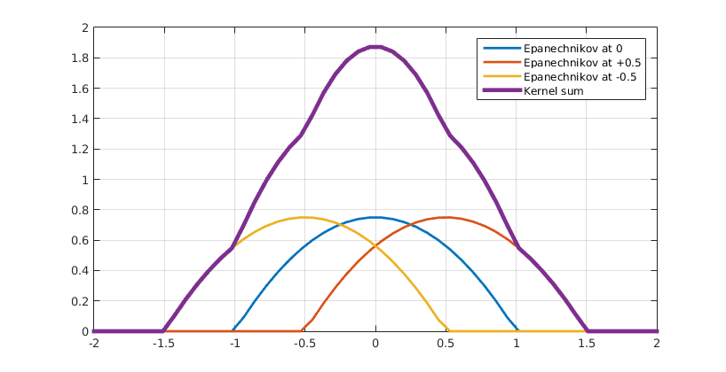
Figure 4 Kernel sum. Click to enlarge
This kernel function can be anything as long is it continuous, symmetric and integrates to 1, since it represents one data point or an agent in our case. Some of the most common kernel functions include gaussian kernels, triangular kernels and epanechnikov kernels. During our simulations we have found the Epanechnikov-Kernel particularly useful. In two dimensions these are defined as: $$k(x,y) = \left\{\begin{matrix} \frac{3}{4h} * (1 - ((x/h)^2 + (y/h)^2)) & \text{if } ((x/h)^2 + (y/h)^2) \leq 1 \\ 0 & \text{else} \end{matrix}\right. $$ Importantly, the scaled functions inherit the kernel function properties, but are either broader or narrower. The degree to which the shape of a kernel function is stretched or squeezed depends on the scaling factor h (fig6), which is why it is called the bandwidth. This parameter gives us the freedom to define how far the influence of an agent reaches and how smooth the resulting density function looks like (fig7 undersmoothed, oversmoothed, ideal). Using a KDE allows us to define the agent density at any point using (Eq. 13).
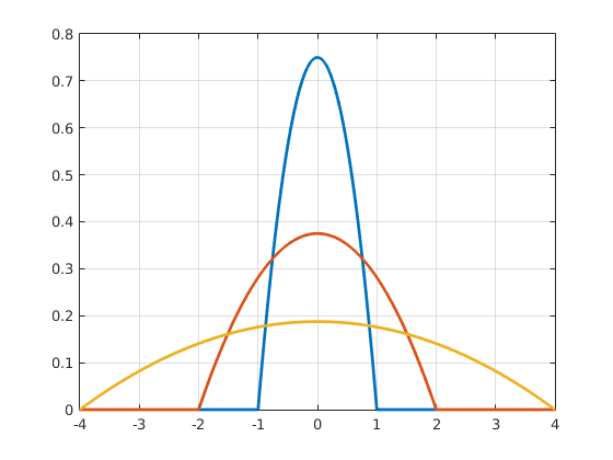
Figure 1 Epanechnikov kernels with bandwidths with various bandwidths. Click to enlarge
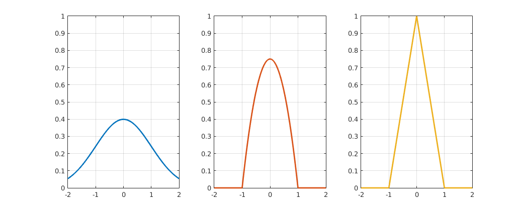
Figure 1 Gaussian, triangular and Epanechnikov kernel functions. Click to enlarge
PDE to agent-based
The final component of our hybrid model is the mapping of the PDE model to the agent-based model.
The latter model works with discrete objects that have continuous coordinates, which means that they can be located
at any point of the domain.
As we have seen, the agents need the local concentration of AHL and leucine, as well as the gradient of leucine in
order to update their positions. In the PDE model however, the domain is discretized into a grid and concentrations
are only defined at grid points. Therefore, in order to transfer information from the PDE model to the agent-based
model we need to translate these grid values into values for any given position within the domain. We achieved this
for the 1-D hybrid model by taking the two nearest grid points to any agent and employing linear interpolation to
derive an approximate local field value. Similarly, for the 2-D hybrid model we took the four nearest grid points
and employed bilinear interpolation, which is explained in box 4. The result is (Eq. 14) to derive the
concentration
or gradient of AHL or leucine at any point in the domain. Taken together, (Eq. 4), (Eq. 11), (Eq. 13) and (Eq. 14)
collectively contain all the PDEs, agent-based SDEs and two-way information transfer functions to fully describe our
hybrid model. All the equations are summarized schematically in (fig8).
Implementation
Agent-based Module
Partial differential equations
As mentioned earlier the concentrations of AHL and Leucine are modeled using partial differential equations.
In the colony level model these equations are solved explicitly. Explicit schemes do not require a lot of
work per time step, but unfortunately are not unconditionally stable. In two dimensions the grid ratios
$dt/dx^2$ and $dt/dy^2$ can not exceed $dt/dx^2 + dt/dy^2 \leq \frac{1}{2}$ for the solver to be stable.
When computing the solution of the hybrid model this requrement forces us to spend a lot of CPU time solving
partial differential equations that could be better spent simulation the agents. Therefore an implicit ADI
Alternating direction implicit scheme has been implemented. ADI-schemes are unconditionally stable, which
allows it to take large time steps with the PDE solver. ADE-schemes are given by the formula:
$$ (1 - \frac{1}{2} \mu_x \delta_x^2) U^{n+\frac{1}{2}} = (1 + \frac{1}{2} \mu_y \delta_y^2) U^n $$
$$ (1 - \frac{1}{2} \mu_y \delta_y^2) U^{n+1} = (1 + \frac{1}{2} \mu_x \delta_x^2)U^{n+\frac{1}{2}} $$
In the equations above $\mu$ denotes grid ratios and $\delta^2$ central differences. The production and
degradation terms have been incorporated at every time level with a factor of $\frac{1}{4}$.
The image below shows the computational molecule of the ADI scheme we chose to implement:

Figure 2 ADI-Molecule. Click to enlarge
Nearest-neightbor Algorithm
Choice of Timestep
Boundary Conditions
Matching
Decoupling of timesteps
In order to benefit from the implicit PDE-solver described above the agent's time steps are chosen smaller
then the time steps of the PDE solver. However type A cells produce molecules continuously as they move
trough space. Therefore we record their positions and average over the kernel functions centered at
past positions since the last PDE evaluation. That way we avoid blurring the results of the PDE solver
too much, when the time step of the agents is reduced.
Last but not least we want to point out the relationship between kernel bandwidth and the grid on which the
PDE is solved. The larger the kernel bandwidth $h$ is chosen the coarser the PDE grid can be without loosing
cells between grid points. If the the diameter of the kernel functions is smaller then the distance between
PDE grid points it can happen, that the kernel does not overlap with any PDE grid points. In this case a cells
contribution to the molecule concentrations at the next time step could be lost. When the PDE grid is
widened to save computing time it is thus necessary to increase the Kernel bandwidth as well. However this
increase can lead to a situation where the Kernel function covers significantly more space then the actual
diameter of a bacterium. In these cases the Kernel function can be interpreted as a probability function for
a cells position. However we avoided too large bandwiths and PDE grids by running our 2-D simulations at the
Flemish Supercomputer Center (VSC).
Figure 3 Logo of the Flemish Supercomputer Center. Click to enlarge
1-D Hybrid Model
The video box above shows one dimensional simulation results for the hybrid model. A constant speed and random step simulation has been computed. We observe that the bacteria form a traveling wave in both cases, which is essential for pattern formation. These results are also similar to what we get from the continuous model, which confirms our results.
2-D Hybrid Model
The videos above show simulation videos computed at the Flemish supercomputing center, for three different initial conditions similar to the ones we used for the colony level model. The first and second condition start from 9 mixed or 5 colonies of both cell types, arranged in a block or star shape. These first two gradually separate in a manner similar to what we would we also saw in the colony level model. The result for random initial data is fundamentally different. As the agent based approach allows for better implementation of adhesion large cell type A bands form. The AHL and Leucine produced by the type A bacteria causes the B type cells to move away leading to a pattern which we could not produce using PDEs alone, this beautifully illustrates the added value of hybrid modeling.
Incorporation of internal model
Up until now, we have largely ignored the inner life of the bacteria. This inner life consists of transcriptional networks and protein kinetics. Instead we assumed that AHL and leucine production is directly proportional to the density of type A cells. This only works in theory, since bacteria will be affected by their surroundings and the way their dynamics react to it. For example bacteria surrounded by a large concentration of AHL, will have more CheZ and will react more on the presence of Leucine. Also bacteria have different histories and will have different levels of transcription factors and different levels of proteins in their plasma. The proteins are not directly degraded and will still be present in the cytoplasm of the bacteria long after the network has been deactivated. From this, it is clear that 2 bacteria, although surrounded by the same AHL and leucine concentrations, can show different behavior and reaction kinetics.
This results in a heterogeneity of the bacterial population that has not yet been accounted for. To make up for this anomaly, we decided to add an internal model to every agent. This way we will get more realistic simulations. Every agent will get their own levels of CheZ, LuxR, LuxI and so on and will have individual reactions on their surroundings. We hope that this way we can get closer to the behavior of real bacteria.
References
| [1] | Benjamin Franz and Radek Erban. Hybrid modelling of individual movement and collective behaviour. Lecture Notes in Mathematics, 2071:129-157, 2013. [ .pdf ] |
| [2] | Zaiyi Guo, Peter M A Sloot, and Joc Cing Tay. A hybrid agent-based approach for modeling microbiological systems. Journal of Theoretical Biology, 255(2):163-175, 2008. [ DOI ] |
| [3] | E F Keller and L A Segel. Traveling bands of chemotactic bacteria: a theoretical analysis. Journal of theoretical biology, 30(2):235-248, 1971. [ DOI ] |
| [4] | E. M. Purcell. Life at low Reynolds number, 1977. [ DOI ] |
| [5] | Angela Stevens. The Derivation of Chemotaxis Equations as Limit Dynamics of Moderately Interacting Stochastic Many-Particle Systems, 2000. [ DOI ] |
Equations


Contact
Address: Celestijnenlaan 200G room 00.08 - 3001 Heverlee
Telephone: +32(0)16 32 73 19
Email: igem@chem.kuleuven.be


