Team:KU Leuven/Modeling/Hybrid

main

Research

Interlab

Modeling

Outreach

Future

Team

Notebook

main

Research

Interlab

Modeling

Outreach

Future

Team

Notebook

$C$: concentration [nmol/cl]
$\vec{r}$: position vector [µm]
$t$: time [h]
$D$: diffusion constant [µm^2/h]

$C$: concentration [nmol/cl]
$\vec{r}$: position vector [µm]
$t$: time [h]
$\alpha$: production constant [nmol/h]
$\rho_A$: density of type A bacteria [#/cl]

$C$: concentration [nmol/cl]
$\vec{r}$: position vector [µm]
$t$: time [h]
$k$: degradation constant [1/h]

$C$: concentration [nmol/cl]
$\vec{r}$: position vector [µm]
$t$: time [h]
$D$: diffusion constant [µm^2/h]
$\alpha$: production constant [nmol/h]
$\rho_A$: density of type A bacteria [#/cl]
$k$: degradation constant [1/h]

$\vec{r}$: position vector [µm]
$t$: time [h]
$\vec{F}_{applied}$: applied force [mN]
$\gamma$: frictional coefficient [mN*h/µm]

$\vec{r}$: position vector [µm]
$t$: time [h]
$\chi$: chemotactic sensitivity [µm^2*cl/(h*nmol)]
$S$: chemoattractant concentration [nmol/cl]
$\mu$: bacteria diffusion constant [µm^2/h]
$\vec{W}$: Wiener process [h^(1/2)]
$\kappa$: chemotactic sensitivity constant [-]

$n$: bacteria density [#/cl]
$\vec{r}$: position vector [µm]
$t$: time [h]
$\mu$: bacteria diffusion constant [µm^2/h]
$\chi$: chemotactic sensitivity [µm^2*cl/(h*nmol)]
$S$: chemoattractant concentration [nmol/cl]
$\kappa$: chemotactic sensitivity coefficient [-]

$\chi$: chemotactic sensitivity [µm^2*cl/(h*nmol)]
$S$: chemoattractant concentration [nmol/cl]
$\mu$: bacteria diffusion constant [µm^2/h]
$\kappa$: chemotactic sensitivity constant [-]
$S$: chemoattractant concentration [nmol/cl]
$\vec{r}$: position vector [µm]
$t$: time [h]

The Hybrid Model

Introduction

The hybrid model represents an intermediate level of detail in between the colony level model and the internal model. Bacteria are treated as individual agents that behave according to Keller-Segel type stochastic differential equations, while chemical species are modeled using partial differential equations. These different models are implemented and coupled within a single hybrid modelling framework.

Partial Differential Equations

Spatial reaction-diffusion models that rely on Partial Differential Equations (PDEs) are based on the assumption that the collective behavior of individual entities, such as molecules or bacteria, can be abstracted to the behavior of a continuous field that represents the density of those entities. The brownian motion of molecules, for instance, is the result of inherently stochastic processes that take place at the individual molecule level, but is modeled at the density level by Fick’s laws of diffusion. These PDE-based models provide a robust method to predict the evolution of large-scale systems, but are only valid when the spatiotemporal scale is sufficiently large to neglect small-scale stochastic fluctuations and physical granularity. Moreover, such a continuous field approximation can only be made if the behavior of the individual entities is well described.

Agent-Based Models

Agent-based models on the other hand explicitly treat the entities as individual “agents” that behave according to a set of “agent rules”. An agent is an object that acts independently from other agents and is influenced only by its local environment. The goal in agent-based models is to study the emergent systems-level properties of a collection of individual agents that follow relatively simple rules. In smoothed particle hydrodynamics for example, fluids are simulated by calculating the trajectory of each individual fluid particle at every timestep. Fluid properties such as the momentum at a certain point can then be sampled by taking a weighted sum of the momenta of the surrounding fluid particles. A large advantage of agent-based models is that the agent rules are arbitrarily complex and thus they allow us to model systems that do not correspond to any existing or easily derivable PDE model. However, because every agent is stored in memory and needs to be processed individually, simulating agent-based models can be computationally intensive.

Hybrid Modeling Framework

In our system, there are both bacteria and chemical species that spread out and interact on a petri dish to form patterns. On the one hand, the bacteria are rather complex entities that move along chemical gradients and interact with one another. Therefore they are ideally modeled using an agent-based model. On the other hand, the diffusion and dynamics of the chemicals leucine and AHL are easily described by well-established PDEs. To make use of the advantages of each modeling approach, we decided to combine these two different types of modeling in a hybrid modeling framework. In this framework we modeled the bacteria as agents, while the chemical species were modeled using PDEs. There were two challenges to our hybrid approach, namely coupling the models and matching them. Coupling refers to the transfer of information between the models and matching refers to dealing with different spatial and temporal scales to achieve accurate, yet computationally tractable simulations.

In the following paragraphs we first introduce our hybrid model and its coupling. Once the basic framework is established, the agent-based module and PDE module are discussed in more depth and the issue of matching is highlighted. We also expand on important aspects of the model and its implementation such as boundary conditions and choice of timesteps. Then the results for the 1-D model and 2-D model simulations are shown and summarized. Finally, the incorporation of the internal model into the hybrid model is discussed and a proof of concept is demonstrated.

Model Description

System

The main protagonists in our pattern-forming system are cell types A and B, AHL and leucine. Cells A produce AHL as well as leucine. They are unaffected by leucine, while cells B are repelled by leucine. AHL modulates the motility of both cell types A and B, but in opposite ways. High concentrations of AHL will render cell type A unable to swim but will activate cell type B’s motility. Conversely, low concentrations of AHL causes swimming of cell type A and incessant tumbling (thus immobility) of cell type B. Lastly, cells A express the adhesin membrane protein, which causes them to stick to each other. Simply said, our system should produce spots of immobile, sticky groups of A type cells, surrounded by rings of B type cells. Any cell that finds itself outside of the region that it should be in, is able to swim to their correct place and becomes immobile there. More details can be found in the research section.

Partial Differential Equations

As discussed in the previous paragraph, our hybrid model incorporates chemical species using PDEs. In our system these are AHL and leucine. The diffusion of AHL and leucine can be described by the heat equation (1).

$$\frac{\partial C(\vec{r},t)}{\partial t}=D \cdot \nabla^2 C(\vec{r},t) \;\;\; \text{(1)}$$

By using (1) we assume that the diffusion speed is isotropic, i.e. the same in all spatial directions. This also explains why it is called the heat equation, since heat diffuses equally fast in all directions. A detailed explanation of the heat equation can be found in box 1. The second factor that needs be taken into account is the production of AHL and leucine by type A bacteria. In principle, AHL and leucine production is dependent on the dynamically-evolving internal states of all cells of type A. However, for our hybrid model we ignored the inner life of all bacteria and instead assumed that AHL and leucine production is directly proportional to the density of A type cells (2).

$$ \frac{\partial C(\vec{r},t)}{\partial t}=\alpha \cdot \rho_A(\vec{r},t) \;\;\; \text{(2)}$$

In the last paragraph we will reconsider this assumption and assign each cell an internal model. Finally, AHL and leucine are organic molecules and therefore they will degrade over time. We assume first-order kinetics meaning that the rate at which AHL and similarly leucine disappear is proportional to their respective concentrations (3a and 3b) assuming neutral pH ^[6].

$$ \frac{\partial C_{AHL}(\vec{r},t)}{\partial t}=-k_{AHL}\cdot C_{AHL}(\vec{r},t) \;\;\; \text{(3a)} $$ $$ \frac{\partial C_{leucine}(\vec{r},t)}{\partial t}=-k_{leucine}\cdot C_{leucine}(\vec{r},t) \;\;\; \text{(3b)} $$

Putting it all together, we obtain (4), both for AHL and leucine.

$$ \frac{\partial C(\vec{r},t)}{\partial t}=D \cdot \nabla^2 C(\vec{r},t)+\alpha \cdot \rho_A(\vec{r},t)-k\cdot C(\vec{r},t) \;\;\; \text{(4)} $$

Note that these equations have exactly the same form as the equations for AHL and leucine in the colony level model. The crucial difference however lies in the calculation of the density of cells of type A. In contrast to the colony level model, the cell density is not calculated explicitly with a PDE and is therefore not trivially known. Therefore a method to extract a density field from a spatial distribution of agents is necessary. This is addressed in the subparagraph below on coupling.

Box 1: Heat Equation

Heat Equation

The left-hand side of the heat equation (1) represents the rate of accumulation of a chemical, while the right-hand side is proportional to the Laplacian of its concentration field, which is a second-order differential operator. This equation can be easily understood by considering a one-dimensional concentration profile, as shown in Figure 1: if the concentration can be approximated as a convex parabolic function, the second derivative is positive and therefore the rate of accumulation is positive (i.e. more accumulation). If on the other hand the concentration resembles a concave parabolic function, the second derivative is negative and the rate of accumulation as well (i.e. depletion). A special case occurs when the concentration profile takes on a linear form. Everything that moves into the point goes out at the other side and as a result there is no net accumulation over time.

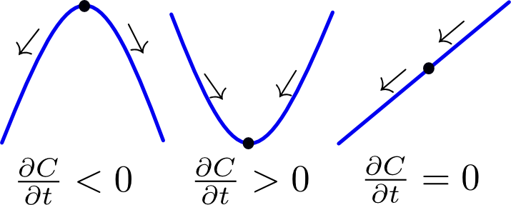
Figure 1
Illustration of the heat equation. Click to enlarge

Agents

To model bacteria movement on the other hand, we used an agent-based model that explicitly stored individual bacteria as agents. Spatial coordinates are associated with each agent, specifying their location. After solving the equation of motion for all agents based on their environment, these coordinates are updated at every timestep. In principle, Newton’s second law of motion has to be solved for all bacteria. However, since bacteria live in a low Reynolds (high friction) environment, the inertia of the bacteria can be neglected. This is because an applied force will immediately be balanced out by an opposing frictional force, with no noticeable acceleration or deceleration phase taking place. This eliminates the inertial term and simplifies Newton’s second law to (5).

$$ \frac{d^2 \vec{r}(t)}{dt^2}=\sum_{i} \vec{F}_{applied,i}-\gamma \cdot \frac{d \vec{r}(t)}{dt}=0 $$ $$\Rightarrow \frac{d \vec{r}(t)}{dt}=\frac{1}{\gamma} \cdot \sum_{i} \vec{F}_{applied,i} \;\;\; \text{(5)} $$

Basically, the velocity can be calculated as the sum of all applied forces times a constant. For more info about the Reynolds number and “life at low Reynolds number”, we refer to box 2.

Stochastic Differential Equation

However, the physical “chemotactic force” that propels bacteria is not easily measured or derived. Therefore, we base the equation of motion in one dimension on (6), a stochastic differential equation (SDE) that describes the motion of a single particle in a N-particle system that is governed by a Keller-Segel type PDE in the limit of $N \rightarrow \infty$. More precisely, the Keller-Segel type PDE (7) describes the evolution of a bacteria density field $n$ with movement towards some chemoattractant $S$.

$$ d\vec{r}_i(t)=\chi (S) \cdot \nabla S(\vec{r},t)\cdot dt + \sqrt{2 \cdot \mu}\cdot d\vec{W} \;\;\; \text{(6a)} $$ $$ d\vec{r}_i(t)=\mu \cdot \frac{\kappa}{S(\vec{r},t)} \cdot \nabla S(\vec{r},t)\cdot dt + \sqrt{2 \cdot \mu}\cdot d\vec{W} \;\;\; \text{(6b)} $$

$$ \frac{\partial n(\vec{r},t)}{\partial t}=\mu \cdot \nabla^2 n - \nabla (n \cdot \chi(S) \cdot\nabla S(\vec{r},t)) \;\;\; \text{(7a)} $$ $$ \frac{\partial n(\vec{r},t)}{\partial t}=\mu \cdot \nabla^2 n - \nabla (n \cdot \mu \cdot \frac{\kappa}{S(\vec{r},t)} \cdot\nabla S(\vec{r},t)) \;\;\; \text{(7b)} $$

Put differently, when infinitely many particles obey (6), they will exhibit Keller-Segel type spatial dynamics as in (7). In a sense, we’re using a “reverse-engineered” particle equation that corresponds to the Keller-Segel field equation. A detailed theoretical treatment of (6) is outside the scope of this model description because it contains a stochastic variable. The traditional rules of calculus do not apply anymore for stochastic differential equations and a different mathematical theory called Itô calculus is required. It is sufficient to say that the second term containing $dW$ accounts for Brownian motion in the form of random noise added to the displacement of the agents, causing them to diffuse, and that it is governed by the diffusion coefficient $\mu$. The first term in (6) on the other hand is easily understood as an advective or drift term (net motion) dependent on S, pushing the agents along a positive gradient (for negative chemotaxis the sign is reversed). The chemotactic force hence points towards an increasing concentration of the chemoattractant. The advective properties are governed by the chemotactic sensitivity function $\chi (S)$. For our model we defined the chemotactic sensitivity function as in (8).

$$ \chi(S)=\mu \cdot \frac{\kappa}{S(\vec{r},t)} \;\;\; \text{(8)} $$

The first important thing to note is that we assumed $\chi (S)$ to be proportional to $1/S$. This is because Keller and Segel proved that their corresponding PDE model only yields travelling wave solutions if $\chi (S)$ contains a singularity at some critical concentration $S_{crit}$, and multiplying by $1/S$ is the simplest way to introduce a singularity at $S_{crit} = 0$. Secondly, the proportionality constant is composed of two factors, namely the bacterial diffusion coefficient $\mu$ and chemotactic sensitivity constant $\kappa$. This is done for two reasons. Firstly, when $\mu$ is lowered, both chemotactic and random motion is reduced, which emulates the state of inactivated motility due to high or low concentrations of AHL. Secondly, defining a separate chemotactic sensitivity constant allows us to examine the effect of the relative strength of chemotaxis versus random motion on pattern formation.

Cell-Cell Interactions

In addition to chemotaxis and diffusion, cell-cell interactions play an important role in pattern formation and also need to be modeled. Bacteria have finite size and therefore multiple bacteria cannot occupy the same space. Moreover, an important mechanism in our system is the aggregation of cells A due to the sticky adhesin protein membrane. To take these mechanisms into account we modeled two types of cell-cell interactions: the purely repulsive interaction of cell B with another cell B and with cell A, and the attractive-repulsive interaction of cell A with another cell A. The interaction between two cells is usually expressed by a potential energy curve defined over the distance between the centers of mass of the two cells (Figure 2).

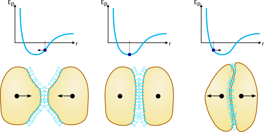
Illustration of cell-cell interaction potential

Figure 2
Cell-cell interaction potential. Click to enlarge

Note that the potential energy remains constant after a certain distance, which means that the cells stop interacting. Also, as two cells move closer together, they hit a wall where the potential energy curve abruptly goes to infinity. The reason for this is that two cells cannot occupy the same space and therefore smaller intercellular distances are not allowed. Implementing this theoretical potential is however not possible because the displacement of bacteria is a stochastic process and the bacteria could randomly jump beyond the potential wall, where the force is ill defined. Therefore, we’ve decided to define a piecewise quadratic potential (9), which results in a piecewise linear force that resembles Hooke’s law, but with three different “spring constants” acting in different intervals of intercellular distances (10).

$$ E_{p,attr-rep}(r_{ij})=\left\{\begin{matrix} 0 & R_{cutoff}\leq r_{ij}\\ -\frac{1}{2}\cdot k_3 \cdot(r_{ij}-R_0)^2 & R_0 \leq r_{ij} < R_{cutoff} \\ -\frac{1}{2}\cdot k_2 \cdot(r_{ij}-R_0)^2 & \frac{R_0}{2} \leq r_{ij} < R_0\\ -\frac{1}{2}\cdot k_1 \cdot(r_{ij}-\frac{k_1+k_2}{k_1}\cdot \frac{R_0}{2})^2 & 0 \leq r_{ij} < \frac{R_0}{2} \end{matrix}\right. \;\;\; \text{(9a)}$$ $$ E_{p,rep}(r_{ij})=\left\{\begin{matrix} 0 & R_0\leq r_{ij}\\ -\frac{1}{2}\cdot k_2 \cdot(r_{ij}-R_0)^2 & \frac{R_0}{2} \leq r_{ij} < R_0\\ -\frac{1}{2}\cdot k_1 \cdot(r_{ij}-\frac{k_1+k_2}{k_1}\cdot \frac{R_0}{2})^2 & 0 \leq r_{ij} < \frac{R_0}{2} \end{matrix}\right. \;\;\; \text{(9b)}$$

$$ \vec{F}_{ij,attr-rep}(r_{ij})= \frac{\partial E_{p,attr-rep}(r_{ij})}{\partial r_{ij}} \cdot \vec{e}_{ij}= \left\{\begin{matrix} \vec{0} & R_{cutoff}\leq r_{ij}\\ k_3 \cdot(r_{ij}-R_0) \cdot \vec{e}_{ij} & R_0 \leq r_{ij} < R_{cutoff} \\ k_2 \cdot(r_{ij}-R_0) \cdot \vec{e}_{ij} &\frac{R_0}{2} \leq r_{ij} < R_0\\ k_1 \cdot(r_{ij}-\frac{k_1+k_2}{k_1}\cdot \frac{R_0}{2}) \cdot \vec{e}_{ij} & 0 \leq r_{ij} < \frac{R_0}{2} \end{matrix}\right. \;\;\; \text{(10a)} $$ $$ \vec{F}_{ij,rep}(r_{ij})= \frac{\partial E_{p,rep}(r_{ij})}{\partial r_{ij}} \cdot \vec{e}_{ij}= \left\{\begin{matrix} \vec{0} & R_0\leq r_{ij}\\ k_2 \cdot(r_{ij}-R_0) \cdot \vec{e}_{ij} & \frac{R_0}{2} \leq r_{ij} < R_0\\ k_1 \cdot(r_{ij}-\frac{k_1+k_2}{k_1}\cdot \frac{R_0}{2}) \cdot \vec{e}_{ij} & 0 \leq r_{ij} < \frac{R_0}{2} \end{matrix}\right. \;\;\; \text{(10b)} $$

Between A type cells, there is a region of attraction $(R_0 \leq r_{ij} < R_{cutoff})$, where the force points towards the other cell, hence moving them closer together. In the repulsive domain $(r_{ij} < R_0)$, two regions were defined, emulating lower repulsive forces $(\frac{R_0}{2} \leq r_{ij} < R_0)$ and higher repulsive forces due to a higher spring constant when the cells are even closer $(r_{ij} < \frac{R_0}{2})$. For the purely repulsive interaction scheme there is no attraction and therefore the spring constant for $R_0 \leq r_{ij}$ is zero. More details about the implementation of the cell-cell interaction scheme, more specifically regarding the nearest-neighbor search algorithm, can be found in the paragraph on the agent-based module below.

Equation of Motion

Now we are ready to construct the equation of motion for cell type A and B as a superposition of the Keller-Segel SDE (6) and the cell interaction forces, yielding (10). $$ d\vec{r}_{A_i}(t)= \sqrt{2 \cdot \mu_A}\cdot d\vec{W} + \frac{1}{\gamma}\cdot\Bigg( \sum^{A \backslash \{ A_i\}}_j \frac{dE_{p,attraction}(r_{ij}(t))}{dr_{ij}}\cdot \vec{e}_{ij}+\sum^{B}_j \frac{dE_{p,repulsion}(r_{ij}(t))}{dr_{ij}}\cdot \vec{e}_{ij} \Bigg)\cdot dt \;\;\; (10a) $$ $$ d\vec{r}_{B_i}(t)= \chi(L(\vec{r},t),H(\vec{r},t)) \cdot \nabla L(\vec{r},t)\cdot dt + \sqrt{2 \cdot \mu_B(H(\vec{r},t))}\cdot d\vec{W} + $$ $$ \frac{1}{\gamma}\cdot\Bigg( \sum^{A\cup B\backslash \{ B_i\}}_j \frac{dE_{p,repulsion}(r_{ij}(t))}{dr_{ij}}\cdot \vec{e}_{ij} \Bigg)\cdot dt $$ $$ \chi(L(\vec{r},t),H(\vec{r},t))= \mu_{B}(H(\vec{r},t)) \cdot \frac{\kappa}{L(\vec{r},t)} $$ $$ \mu_A(H(\vec{r},t))=\left\{\begin{matrix}\mu_{A,high} & H(\vec{r},t) < H_{A,threshold}\\ \mu_{A,low} & H(\vec{r},t) \geq H_{A,threshold}\end{matrix}\right. $$ $$ \mu_B(H(\vec{r},t))=\left\{\begin{matrix} \mu_{B,high} & H(\vec{r},t) < H_{B,threshold}\\ \mu_{B,low} & H(\vec{r},t) \geq H_{B,threshold} \end{matrix}\right. \;\;\; \text{(10b)} $$ Bacteria of type A are not attracted nor repelled by leucine, so the chemotactic term falls away. All cell-cell forces are summed up to find a net force, taking into account the two different potentials due to the different interaction types. As discussed before, this net force times a constant yields the velocity due to that force, which is then multiplied by dt to obtain the displacement. For B type cells, the chemotactic term models the repulsive chemotaxis away from leucine. The chemotactic sensitivity function has a negative sign signifying that B type cells are repelled by leucine. The cell interaction term in this case is simpler because B type cells only interact repulsively. Note that the diffusion coefficient of cell types A and B switches based on the local concentration of AHL relative to a threshold AHL value, which simulates the dependency of cellular motility on AHL. The agent-based module is now fully defined but one crucial issue was skipped: AHL and leucine concentrations are calculated using PDEs and are therefore only known at grid points. Agents on the other hand reside in the space between grid points and require local concentrations as inputs to calculate their next step. This problem is part of the coupling aspect in our hybrid modeling framework and is discussed below.

Coupling

Introductory text about coupling.

Agent-based to PDE

As described above, the agents’ effect in the PDE is modeled as a source term that is proportional to the agent density. This approach is essentially the same approach taken in the colony level model for the bacterial production of AHL and leucine. However, in the colony level model the bacteria density is explicitly calculated at the grid points, while the agent-based model essentially considers a set of points in space. A simple first-order approach would be to determine the closest grid point to any agent and simply increment a counter belonging to that grid point. This results in a histogram, which can be used directly to represent the agent density. However, the resulting density is a blocky, nonsmooth function which poorly represents the underlying agent distribution. The effect of a single agent is artificially confined to a single grid point, while in reality an agent’s influence could reach much further than a single grid point. The shape of a histogram is also very dependent on the bin size, which in this case corresponds to the grid spacing so it cannot be independently tuned. To decouple grid spacing and agent density and achieve a smoother density function, we made use of a more sophisticated technique called kernel density estimation (KDE).

KDE is used in statistics to estimate the probability density of a set discrete data derived from a random process. The basic idea consists of defining a kernel function that represents the density of a single data point, then centering kernel functions on every data point and summing them all up to achieve a smooth overall density function, as demonstrated in the figure below.

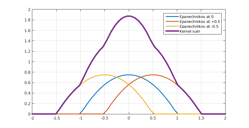
Figure 2
Kernel sum. Click to enlarge

This kernel function can be anything as long is it continuous, symmetric and integrates to 1, since it represents one data point or an agent in our case. Some of the most common kernel functions include gaussian kernels, triangular kernels and epanechnikov kernels. During our simulations we have found the epanechnikov kernel particularly useful. In two dimensions these are defined as: $$k(x,y) = \left\{\begin{matrix} \frac{3}{4h} * (1 - ((x/h)^2 + (y/h)^2)) & \text{if } ((x/h)^2 + (y/h)^2) \leq 1 \\ 0 & \text{else} \end{matrix}\right. \;\;\; (11) $$ Importantly, the scaled functions inherit the kernel function properties, but are either broader or narrower. The degree to which the shape of a kernel function is stretched or squeezed depends on the scaling factor h , which is why it is called the bandwidth. This parameter gives us the freedom to define how far the influence of an agent reaches and how smooth the resulting density function looks like. Using a KDE allows us to define the agent density at any point by referring to the kernel sum.

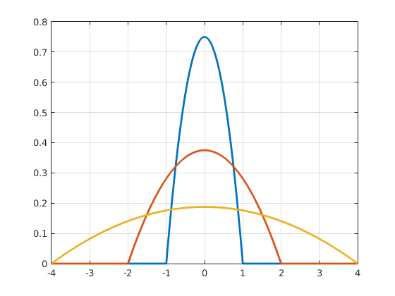
Figure 3
Epanechnikov kernels with bandwidths with various bandwidths. Click to enlarge

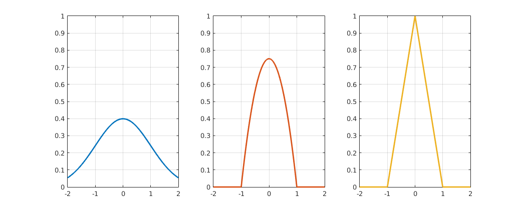
Figure 4
Gaussian, triangular and Epanechnikov kernel functions. Click to enlarge

PDE to agent-based

The final component of our hybrid model is the mapping of the PDE model to the agent-based model. The latter model works with discrete objects that have continuous coordinates, which means that they can be located at any point of the domain. As we have seen, the agents need the local concentration of AHL and leucine, as well as the gradient of leucine in order to update their positions. In the PDE model however, the domain is discretized into a grid and concentrations are only defined at grid points. Therefore, in order to transfer information from the PDE model to the agent-based model we need to translate these grid values into values for any given position within the domain. We achieved this for the 1-D hybrid model by taking the two nearest grid points to any agent and employing linear interpolation to derive an approximate local field value. Similarly, for the 2-D hybrid model we took the four nearest grid points and employed bilinear interpolation.

Implementation

Agent-Based Module

Introductory text about the Agent-Based Module

Nearest-Neighbor Algorithm

The cell-cell interactions have already been fully described in the paragraphs above. However, solving the equation of motion of an agent in its current form requires the computation of the force due to every other agent. If we take N to be the number of agents, that means $N*(N-1)$ amount of force computations are needed in total and therefore the computation time grows as $O(N^2)$. To put this in perspective, if we simulate a thousand agents, the amount of interactions adds up to around one million. This puts a heavy computational load on the model which can be reduced greatly by using a smarter algorithm. The crucial observation here is that the force goes to zero when the distance between two cells is larger than $2\cdot r_{cutoff}$. An agent therefore only interacts with its nearest neighbors, meaning that the naive implementation wastes a lot of time computing interactions which have no effect anyways. Moreover, as the simulation progresses, an agent’s neighbors do not vary greatly from one timestep to another. A more efficient approach then consists of periodically searching for the nearest neighbors within a fixed radius, storing them in a list for every agent and updating their coordinates for all intermediate timesteps. Since the agents are programmed to repel each other when they approach each other too closely, they will evolve to a rather uniform distribution. The most appropriate fixed-radius nearest neighbor search algorithm in that case is the cell technique. In this algorithm, the agents are structured by placing a rectangular grid of cells over the domain and assigning every agent to a cell (fig9). Determining which cell an agent belongs to is easily done by rounding down the x and y-coordinates to the nearest multiple of the grid spacing. If the grid spacing is chosen so that interactions do not reach further than adjacent cells, every agent only needs to look for neighbors in 9 cells (its own cells plus 8 adjacent cells) instead of the entire domain.

Choice of timestep

In contrast to PDE models, there is no danger of instability due to a large timestep in agent-based models. However, since the time step determines how far a cell can “jump” away from its previous position, we need to ensure that it is not so large as to negate the effect of intercellular interactions. To understand this, we first discretize the Brownian motion term in the agent’s equation of motion (eq. 15). It can be proven that this term follows a distribution as (eq. 16). Now assume that there are two A type cells who are exactly 2*r0 apart. If the timestep is too large, they might “jump” out of each other’s influence at the next iteration. This situation is highly unrealistic because the cells actually should feel each other’s pull while they randomly drift away from each other. If the timestep is too large, there’s a high probability that the cells detach without experiencing the potential at all and therefore the probability of detachment is artificially inflated. Of course, we can never completely eliminate the possibility of a sudden detachment because the random is sampled by a normal distribution, but we can define a desired probability of sudden detachment P-. Then, for a given r0, rcutoff and µA, we can determine how small the timestep has to be for the sudden detachment to happen only with probability P-. First, we assume two A type cells with coordinates (x1,y1) and (x2,y2) that are at a distance 2*r0 = R0 from each other. We then define the coordinates at the next timestep as stochastic variables X1, Y1, X2 and Y2, which are distributed as (eq. 17). We are not interested in the future coordinates as such, but rather in the future intercellular distance, which is composed of these future coordinates and therefore also is a stochastic variable. For ease of calculation, we work with the square of this variable, which we name as R² and define as (eq. 18). It is easy to see that X1-X2 and Y1-Y2 are both noncentral (mean is not equal to zero) normally distributed variables as well. Therefore R² obeys a noncentral chi-squared distribution with 2 degrees of freedom. Before proceeding further, we have to make our R² conform to a standard noncentral chi-squared distribution. First we normalize X1-X2 and Y1-Y2. We observe that X1-X2 and Y1-Y2 are distributed as (eq. 19). Secondly, because the means of the X1-X2 and Y1-Y2 are not equal to zero, we need to account for this by calculating the noncentrality parameter \lambda. This is equal to the sum of squares of the means of the normalized X1-X2 and Y1-Y2 variables, which of course equals (eq. 20), corresponding to a scaled version of the original intercellular distance. We then define the standardized variable R’² as (eq. 21). To recap, the meaning of R’² is the scaled squared intercellular distance after updating once with timestep \triangle t starting from an initial distance of R0. Then we define F as the cumulative distribution function (eq. 22). To then finally calculate appropriate timestep for a given r0, rcutoff and µA we take the inverse cumulative distribution function and equate it to the scaled squared intercellular cutoff distance (eq. 23). Note that both the left hand side and right hand side depend on the \triangle t in a nonlinear way, therefore a nonlinear solver is required.

Partial Differential Equations Module

Introductory text about the Partial Differential Equations Module

Computational Scheme

As mentioned earlier the concentrations of AHL and Leucine are modeled using partial differential equations. In the colony level model these equations are solved explicitly. Explicit schemes do not require a lot of work per time step, but unfortunately are not unconditionally stable. In two dimensions the grid ratios $dt/dx^2$ and $dt/dy^2$ can not exceed $dt/dx^2 + dt/dy^2 \leq \frac{1}{2}$ for the solver to be stable. When computing the solution of the hybrid model this requrement forces us to spend a lot of CPU time solving partial differential equations that could be better spent simulation the agents. Therefore an implicit ADI Alternating direction implicit scheme has been implemented. ADI-schemes are unconditionally stable, which allows it to take large time steps with the PDE solver. We used the following scheme: $$ (1 - \frac{1}{2} \mu_x \delta_x^2) U^{n+\frac{1}{2}} + \frac{1}{4}kU^{n+\frac{1}{2}} = (1 + \frac{1}{2} \mu_y \delta_y^2) U^n - \frac{1}{4}kU^n + \frac{\alpha}{2} \rho_A $$ $$ (1 - \frac{1}{2} \mu_y \delta_y^2) U^{n+1} + \frac{1}{4}kU^{n+1} = (1 + \frac{1}{2} \mu_x \delta_x^2)U^{n+\frac{1}{2}} - \frac{1}{4}kU^{n+\frac{1}{2}} + \frac{\alpha}{2} \rho_A $$ In the equations above $\mu$ denotes grid ratios and $\delta^2$ central differences. The production and degradation terms have been incorporated at every time level with a factor of $\frac{1}{4}$. The image below shows the computational molecule of the ADI scheme we chose to implement:

Figure 4
ADI-Molecule. Click to enlarge

Boundary conditions

Text about boundary conditions.

Matching

Introductory text about matching

Decoupling of timesteps

In order to benefit from the implicit PDE-solver described above the agent's time steps are chosen smaller then the time steps of the PDE solver. However type A cells produce molecules continuously as they move trough space. Therefore we record their positions and average over the kernel functions centered at past positions since the last PDE evaluation. That way we avoid blurring the results of the PDE solver too much, when the time step of the agents is reduced. Last but not least we want to point out the relationship between kernel bandwidth and the grid on which the PDE is solved. The larger the kernel bandwidth $h$ is chosen the coarser the PDE grid can be without loosing cells between grid points. If the the diameter of the kernel functions is smaller then the distance between PDE grid points it can happen, that the kernel does not overlap with any PDE grid points. In this case a cells contribution to the molecule concentrations at the next time step could be lost. When the PDE grid is widened to save computing time it is thus necessary to increase the Kernel bandwidth as well. However this increase can lead to a situation where the Kernel function covers significantly more space then the actual diameter of a bacterium. In these cases the Kernel function can be interpreted as a probability function for a cells position. However we avoided too large bandwiths and PDE grids by running our 2-D simulations at the Flemish Supercomputer Center (VSC).

Figure 6
Logo of the Flemish Supercomputer Center. Click to enlarge

Bandwidth tuning

Text about bandwidth tuning.

1-D Hybrid Model

The video box above shows one dimensional simulation results for the hybrid model. A constant speed and random step simulation has been computed. We observe that the bacteria form a traveling wave in both cases, which is essential for pattern formation. These results are also similar to what we get from the continuous model, which confirms our results.

2-D Hybrid Model

The videos above show simulation videos computed at the Flemish supercomputing center, for three different initial conditions similar to the ones we used for the colony level model. The first and second condition start from 9 mixed or 5 colonies of both cell types, arranged in a block or star shape. These first two gradually separate in a manner similar to what we would we also saw in the colony level model. The result for random initial data is fundamentally different. As the agent based approach allows for better implementation of adhesion large cell type A bands form. The AHL and Leucine produced by the type A bacteria causes the B type cells to move away leading to a pattern which we could not produce using PDEs alone, this beautifully illustrates the added value of hybrid modeling.

Incorporation of internal model

Up until now, we have largely ignored the inner life of the bacteria. This inner life consists of transcriptional networks and protein kinetics. Instead we assumed that AHL and leucine production is directly proportional to the density of type A cells. This only works in theory, since bacteria will be affected by their surroundings and the way their dynamics react to it. For example bacteria surrounded by a large concentration of AHL, will have more CheZ and will react more on the presence of Leucine. Also bacteria have different histories and will have different levels of transcription factors and different levels of proteins in their plasma. The proteins are not directly degraded and will still be present in the cytoplasm of the bacteria long after the network has been deactivated. From this, it is clear that 2 bacteria, although surrounded by the same AHL and leucine concentrations, can show different behavior and reaction kinetics.

This results in a heterogeneity of the bacterial population that has not yet been accounted for. To make up for this anomaly, we decided to add an internal model to every agent. This way we will get more realistic simulations. Every agent will get their own levels of CheZ, LuxR, LuxI and so on and will have individual reactions on their surroundings. We hope that this way we can get closer to the behavior of real bacteria.

References

[1]	Benjamin Franz and Radek Erban. Hybrid modelling of individual movement and collective behaviour. Lecture Notes in Mathematics, 2071:129-157, 2013. [ .pdf ]
[2]	Zaiyi Guo, Peter M A Sloot, and Joc Cing Tay. A hybrid agent-based approach for modeling microbiological systems. Journal of Theoretical Biology, 255(2):163-175, 2008. [ DOI ]
[3]	E F Keller and L A Segel. Traveling bands of chemotactic bacteria: a theoretical analysis. Journal of theoretical biology, 30(2):235-248, 1971. [ DOI ]
[4]	E. M. Purcell. Life at low Reynolds number, 1977. [ DOI ]
[5]	Angela Stevens. The Derivation of Chemotaxis Equations as Limit Dynamics of Moderately Interacting Stochastic Many-Particle Systems, 2000. [ DOI ]
[6]	A. L. Schaefer, B. L. Hanzelka, M. R. Parsek, and E. P. Greenberg. Detection, purification, and structural elucidation of the acylhomoserine lactone inducer of Vibrio fischeri luminescence and other related molecules. Bioluminescence and Chemiluminescence, Pt C, 305:288-301, 2000.