Team:Exeter/Modeling

Modelling

Introduction

Modelling is a fundamental part of our project, it allows us to not only test our system rigorously but also provide a visual output to make it easier to see what is going on. The purpose of the model is to mainly inform the lab team and improve and compliment their experimental design.

Our model is designed around a MatLab based physical simulation, contained within a microcentrifuge tube that we will use in testing. MatLab was chosen as the programming language of choice as we had all used it before and were comfortable with it.

Our model is built up from two parts:

• A system simulation designed in MatLab, enabling a visual demonstration of the system as well as assisting in the second part.
• Graphical output of parameter scanning developed from the MatLab simulation. This allowed us to check each input variable over a wide range of values so that we could determine the optimum experimental range of each.

We also aim to build a mathematical model to perform parameter scanning, this would then be compared with the simulation based model.

Producing a graphical and numerical output allows us both to establish the controlling factors in our experiment, and to understand the mechanisms of the system. Parameter scanning lets us inform the lab team of the optimal parameter values as well as what parameters can be left alone. By using two methods of parameter scanning we can compare these and hence improve the data given to the lab team.

Simulation

The idea for the model was conceived within the first week after choosing our project. It was based on the idea that the particles would behave in a random motion similar to that of Brownian motion.

We chose to use Matlab, as it was the only one that every member of the modelling team had previously used. This allowed us to start work on it right away as we did not need to learn a whole new computer language.

The fundamental idea was to have two types of particles on a random walk which could then interact with each other if they came close enough. These two particles would be the RNA trigger and the Toehold switch.

The aim of this would be to provide a visual output so that people could see what was going on within our physical system. So in effect we would be creating a simulation of our system. This drove the model in the beginning as we started to try and implement as many real world features as we could, to get the most accurate simulation.

The first of these features was to make something happen when the trigger and switch got close enough to bind hence forming a complex. We made them join together irreversibly, this was primitive but allowed us to forge ahead. The next feature was to make the simulation 3D. This was achieved relatively easily.

After consulting with the lab team we had even more to add to our model. The first thing that needed to be implemented was to allow the complex to break apart after being joined for a period of time. This was to fix the primitive nature of the permanent binding and more accurately reflect the mechanisms inside the system. Next a spherical area of binding was added to replace the cube previously used. This means that the trigger and switch have two spheres at either end which if overlapping, results in their binding. This simulated the spherical area of influence which we estimated to be around the trigger and switch.

A spherical area of influence was used after a discussion with Prof Peter Winlove, we asked him if it would be possible determine the actual size of the trigger and switch, he said this would not be possible. Instead he suggested that we estimate the size of the molecules and assume a sphere around it in which interactions will occur.

INSERT A BIT ABOUT THE MATHS USED FOR THE TWO INTERACTING SPHERES.

****Therefore we decided that the best way to implement this into our simulation was to use binding distance A, which represented the radius of the sphere in which interactions occur. We then compared the distance between two particles and if the distance was shorter than 2A (for the two radii of the interaction spheres of the particles) then the two particles have a chance of joining – Later this would be controlled by a probability function derived from in silico data from NUPACK of the free energies of the complexed and uncomplexed structures.****

Once this was achieved the simulation acted reasonably like the real world system. To improve a lot of research was done to try and find out real world values to add into the simulation. These included particle diameters, binding distances, viscosities, temperatures, etc. After speaking to an advisor we decided to use low binding affinity tubes, allowing us to negate any binding interaction with the walls of the tube. This information was needed so we could figure out what happened to the particles at the wall of the tube containing our sample.

Now we had all the information needed we could confine it to the tube. After consulting with the lab team we chose a 1.5ml microcentrifuge tube. Initially we set up to confine it to a cylinder with the volume equal to the tube. The idea was that, by adding in a confinement element, we could simulate the interaction between the walls of the tube and the particles. Initially we just made it so if they left the tube the particles were placed at its edge. This was a basic step, with the thinking being we would add in a rebound function later.

INSERT THE MATHS ON CALCULATING IF IT HAS LEFT THE TUBE

For determining whether a particle had left the tube or not, we designed a function named ‘checkxy’ to check whether the x and y coordinates generated were outside of the confining container. This was achieved by using manufacturer’s specifications documents to obtain a radius for the container, initially an Eppendorf microcentrifuge tube. In its infancy the function simply compared the coordinates to the radius of the container and if found to be outside, reset the respective breaching coordinate to the boundary of the container by setting it equal to the radius. However we quickly realised in incorrectness in this procedure. Instead, after many diagrams and conversations about the trigonometry of the issue, we settled on a method that calculated the equation of the line from the origin to the external point, and then truncated this line at a distance equal to the radius of the circle to find roughly, the point of exit. This function would later be expanded to deal with the bouncing of particles away from the edge of the system.

After a meeting with a computer scientist at our University, Dr Jonathan Fieldsend, we set about improving our code. The plan was to implement a new coordinate generation system, change the confinement, and finally separate into functions. The plan was first thought out on paper, we then tried to implement this.

The first thing we did was to change the coordinate generation so that it happens on every time step rather than all at once at the beginning. This means that we only need to pass two sets of coordinates between each function per time step, hence speeding up or code. After this a speed test of the code was performed and this decreased the compiling speed by around a half. Another benefit of this generation was that we could store the coordinate into an array which we could then use for many different reasons after the generation had happened. These included producing the 3D simulation and the numerical output.

Once the coordinates had been simplified splitting the code into separate functions also became a lot easier. This was due to the fact only one vector (with the coordinates of the current and previous timesteps) needed to be passed between the functions. The code was split based on the functions that they performed, such as plotting and confinement. This was a serious undertaking and took a lot longer than expected. Our Matlab skills were stretched and a lot of trial and error was needed to make the functions work as expected.

The confinement was changed so that it more accurately mimicked a microcentrifuge tube, this was achieved by altering the cylinder previously used and adding a cone to the base. The cone presented an issue as the radius will not be constant along its height, this required the radius to be calculated ad hoc.

INSERT BIT ABOUT THE CONE RADIUS MATHS

****After deciding that confinement to a microcentrifuge tube was what we wanted, we worked on calculating the cone radius at any given height within the conical aspect of the tube. According to the technical specifications, the radius in the cylindrical aspect is not uniform, however we considered to as a perfect cylinder for the ease of simulation.

For the conical component however, we calculated the equation of the slope in the cone in r (radius = √ x² + y²  ) and z as shown below:

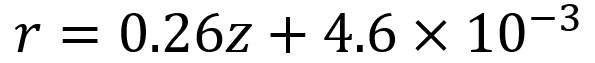
Using this, we could therefore find the radius at any given height within the conical region, given a z coordinate. This would prove to be more difficult when the bouncing and trajectory maths was considered later.

After all of the changes Jonathan suggested had been implemented a lot of debugging and optimisation occurred. This was jointly to do with our coding skills improving, our coding skills being tested, and more input from academics. We optimised loops, variables and functions; added in a cool down period and a requirement that the trigger and switch bind for at least one time step.

The benefit of all of this work was that now the code is separated into functions debugging can occur quicker, the code is simpler and more efficient, and finally it gives us the freedom to choose what output we like. We can either use the random walks to produce a visual simulation or a numerical output which when combined with parameter scanning can be a powerful tool.