Team:Exeter/Modeling
Modelling
Introduction
Modelling is a fundamental part of our project, it allows us to not only test our system rigorously but also provide a visual output to make it easier to see what is going on. The purpose of the model is to mainly inform the lab team and improve and compliment their experimental design.
Our model is designed around a MatLab based physical simulation, contained within a microcentrifuge tube that we will use in testing. MatLab was chosen as the programming language of choice as we had all used it before and were comfortable with it.
Our model is built up from two parts:
- A system simulation designed in MatLab, enabling a visual demonstration of the system as well as assisting in the second part.
- Graphical output of parameter scanning developed from the MatLab simulation. This allowed us to check each input variable over a wide range of values so that we could determine the optimum experimental range of each.
We also aim to build a mathematical model to perform parameter scanning, this would then be compared with the simulation based model.
Producing a graphical and numerical output allows us both to establish the controlling factors in our experiment, and to understand the mechanisms of the system. Parameter scanning lets us inform the lab team of the optimal parameter values as well as what parameters can be left alone. By using two methods of parameter scanning we can compare these and hence improve the data given to the lab team.
Key Meetings
Jonathan prompted many conversations about our model and the assumptions made when designing it. We had two very in depth meetings with him, the first involved a significant restructure and the second to follow up on this. We have since significantly altered the code to accommodate these changes, this is a quick summary of those changes.
In the first meeting, Jonathan questioned some aspects of the model:
- The particles’ interaction with the boundary - to answer this we spoke to another academic Dr Nic Harmer, he informed us that if we could source low binding affinity consumables then we could assume the particles just bounce freely off the walls.
- Whether the particles’ speed is continuous - we decided we could slow the particles down at each time step by reducing the range of the random number generator.
- How different variables, such as temperature, affect the model - we developed parameter scanning to help answer this.
This meeting caused a significant restructuring of our code following Jonathan’s help in improving our matlab practices and his tips on how to speed up our code. These are discussed in greater detail in the simulation section.
The follow up meeting discussed a huge range of topics, Dr Tom Howard also sat in on this and added to the conversation by trying to see the application to the ‘wet’ lab. The topics included more code optimisation, publishing our code, outputs, and the lab application.
The second two points link together as we altered our code to provide a numerical output so that it could be transformed into a parameter scanning function. Tom had a great deal of input on this pointing out which parameters we would need to scan and why. This is outlined further in the parameter scanning section.
Simulation
Initial Ideas
The idea for the model was conceived within the first week after choosing our project. It was based on the idea that the particles would behave in a random motion similar to that of Brownian motion.
We chose to use Matlab, as it was the only program that every member of the modelling team had previously used. This allowed us to start work on it right away as we did not need to learn a whole new computer language.
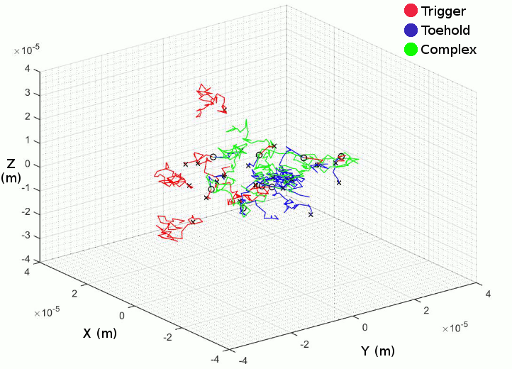
The fundamental idea was to have two types of particles on a random walk which could then interact with each other if they came close enough. These two particles would be the RNA trigger and the Toehold switch.
The aim of this would be to provide a visual output so that people could see what was going on within our physical system. So in effect we would be creating a simulation of our system. This drove the model in the beginning as we started to try and implement as many real world features as we could, to get the most accurate simulation.
Primary Features

The first of these features was to simulate the interaction between the trigger and switch after they get close enough to bind, hence forming a complex. We made them join together irreversibly, a primitive approach but it allowed us to forge ahead. The next feature was to make the simulation 3D which was achieved relatively easily.
Further Additions
After consulting with the lab team we had even more to add to our model. The first thing that needed to be implemented was allowing the complex to break apart after being joined for a period of time. This was to fix the primitive nature of the permanent binding and more accurately reflect the mechanisms inside the system. Next, a spherical area of binding was added to replace the cube previously used - the trigger and switch have two spheres at either end which if overlapping, results in their binding. This simulated the spherical area of influence which we estimated to be around the trigger and switch.
A spherical area of influence was used after a discussion with Prof Peter Winlove. We asked him if it would be possible determine the actual size of the trigger and switch which he said it would not be possible, in our time frame. Instead he suggested that we estimate the size of the molecules and assume a sphere around each in which interactions occur.
We decided that the best way to implement this into our simulation was to use a binding distance A, which represented the radius of the sphere in which interactions occur. We then compared the distance between two particles and if the distance was shorter than 2A (for the two radii of the interaction spheres of the particles) then the two particles have a chance of joining – Later this would be controlled by a probability function derived from in silico data from NUPACK of the free energies of the complexed and uncomplexed structures.
Making Our Simulation Realistic
Once this was achieved the simulation acted reasonably like the real world system. To improve, a lot of research was done into finding out real world values to add into the simulation. These included particle diameters, binding distances, viscosities, temperatures, etc. After speaking to an advisor, Dr Nic Harmer, we decided to use low binding affinity tubes, allowing us to negate any binding interaction with the walls of the tube. This information was needed so we could figure out what happened to the particles at the wall of the tube containing our sample.
Confinement
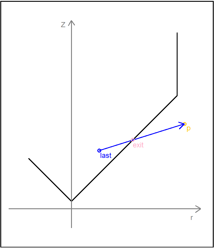
Now we had all the information needed we could confine our simulation to the tube. After consulting with the lab team we chose a 1.5ml microcentrifuge tube. Initially we confined it to a cylinder with the volume equal to the tube. By adding in a confinement element, we could simulate the interaction between the walls of the tube and the particles. Initially, if the particles left the tube they were simply placed at its edge. This was a basic step, with the thinking being we would add in a rebound function later, as you can see in the image below which shows the progression of our design.
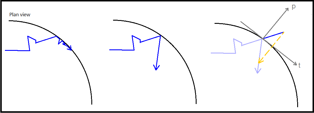
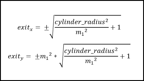
To determine whether a particle had left the tube or not, we designed a function named ‘checkxy’ to check whether the x and y coordinates generated were outside of the confining container. This was achieved by using manufacturer’s specifications documents to obtain a radius for the container, initially an Eppendorf microcentrifuge tube. In its infancy the function simply compared the coordinates of the particle to the radius of the container and if found to be outside, reset the respective breaching coordinate to the boundary of the container by setting it equal to the radius. However we quickly realised the inaccuracy in this procedure. Instead, after many diagrams and conversations about the trigonometry of the issue, we settled on a method that calculated the equation of the line from the origin to the external point, and then truncated this line at a distance equal to the radius of the circle to find roughly, the point of exit. This function would later be expanded to deal with the bouncing of particles away from the edge of the system.
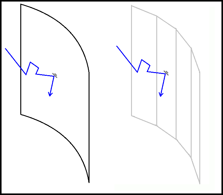
This diagram shows that the boundary of the tube, whilst assumed to be circular would infact be made up of a series of “flat panels” that form the overall cylindrical shape of the container wall.
The previous diagram also shows the rebounding of the particle, crucial for which are the calculations of the coordinates of the exit point. ExitZ calculation is explained later on.
Tidying Up The Code
After a meeting with a computer scientist at our University, Dr Jonathan Fieldsend, we set about improving our code. The plan was to implement a new coordinate generation system, change the confinement, and finally separate into functions. First putting our ideas to paper, we then tried to implement these.
Initially we changed the coordinate generation so that it happened on every time step rather than all at once at the beginning. This meant that we only need to pass two sets of coordinates between each function per time step, hence speeding up our code. Speed tests of the code suggested this decreased the compiling speed by around a half. Another benefit of this generation method was that we could store the coordinates into an array which could then be used for many different purposes after the generation had happened. These included producing the 3D simulation and the numerical output.
Once the coordinates had been simplified splitting the code into separate functions also became a lot easier. This was due to the fact only one vector (with the coordinates of the current and previous timesteps) needed to be passed between the functions. The code was split based on the functions that they performed, such as plotting and confinement. This was a serious undertaking and took a lot longer than expected. Our Matlab skills were stretched and a lot of trial and error was needed to make the functions work as expected.
More Confinement Changes
The confinement was changed so that it more accurately mimicked a microcentrifuge tube This was achieved by altering the cylinder previously used and adding a cone to the base. The cone presented an issue as the radius was not constant along its height requiring the radius to be calculated ad hoc.
After deciding that confinement to a microcentrifuge tube was what we wanted, we worked on calculating the cone radius at any given height within the conical aspect of the tube. According to the technical specifications, the radius in the cylindrical aspect is not uniform, however we considered to as a perfect cylinder for the ease of simulation.
For the conical component, we calculated the equation of the slope in the cone in r (radius = √ x2 + y2 ) and z as shown below:
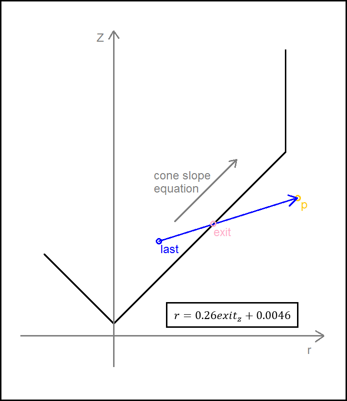
Using this, we could therefore find the radius at any given height within the conical region, given a z coordinate. This would prove to be more difficult when the bouncing and trajectory maths was considered later.
Little Tweaks
After all of the changes Jonathan suggested had been implemented, a lot of debugging and optimisation occurred. This was due to our coding skills improving and being tested, and more input from academics. We optimised loops, variables and functions; added in a cool down period and a requirement that the trigger and switch bind for at least one time step.
The benefit of all of this work was that with the code separated into functions debugging can occur quicker, the code is simpler and more efficient, and finally it gives us the freedom to choose the output. We can either use the random walks to produce a visual simulation or a numerical output which when combined with parameter scanning can be a powerful tool.
New Features
Two new features were worked on in tandem, these are parameter scanning and a trajectory/collision function for the interaction of particles with the walls of the chamber.
Trajectory Calculations at Boundaries of System
Two Dimensions
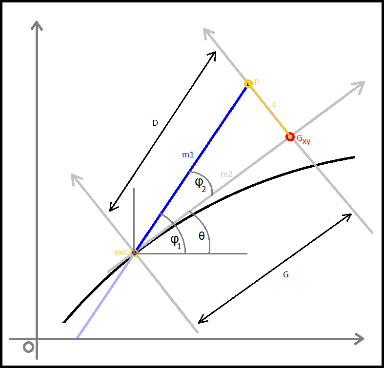
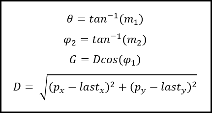
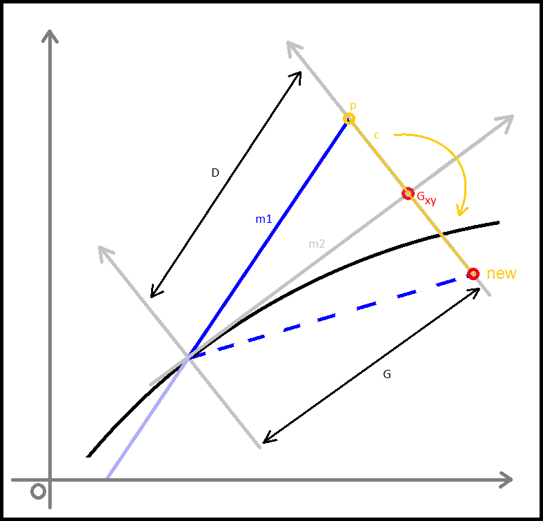
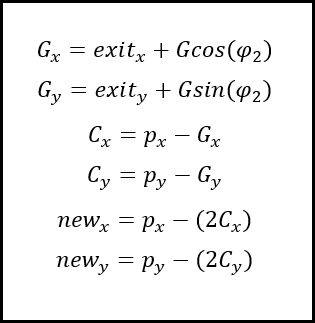
Alteration of the checkxy function to incorporate the bouncing code was therefore undertaken. We worked primarily to determine the trajectory of the particle on its path outside of the tube. Logically we calculated the equation of the line of travel (from last to p) as well as the equation of the tangential line at the point of exit from the container. The next step was to calculate the angle between these two lines and using this, determine the lengths (or velocities) of the path past the breach point in terms of perpendicular and tangential components. To do this, we employed some simple trigonometry that enabled the evalution of the new point that remained inside the container.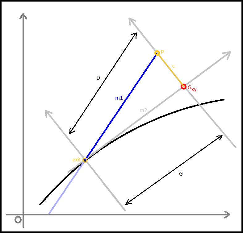
Three Dimensions
The difference in the three dimensional component; the values separating the consecutive z-coordinates of each path are unaffected by the impact and reflection that occur at the boundaries of our container, other than at the top and bottom interfaces, where reflection inverse to the prior z-velocity would occur. This was relatively easy to implement as it was simply a continuation of previous trajectory in the z-axis.
In the cone region
We then faced a significant challenge when we began to consider the alterations of trajectory in the simplified conical region of the container we had initially intended to use, a micro-centrifuge tube.
After these features were implemented we changed the confinement shape away from this and back to a cylinder. This choice was made after discussions with the lab team as they had decided to change their experiments to a micro well plate. A cylinder better reflects this shape and hence the application of the model to the lab.
In the future, we would hope that we/future teams would successfully achieve the development of trajectory calculating code for non-cylindrical containers, as this would enable for simulating in containers that better reflect how a cell free system would behave in a functional prototype.
NUPACK Validation
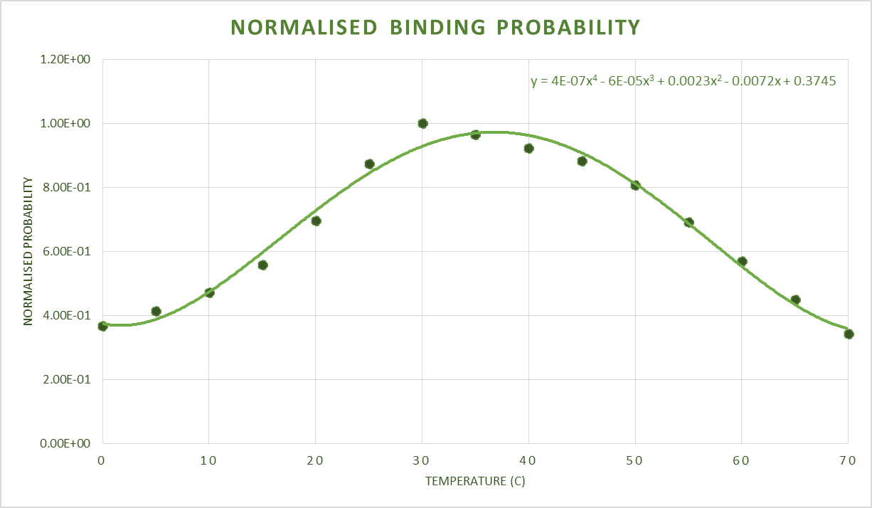
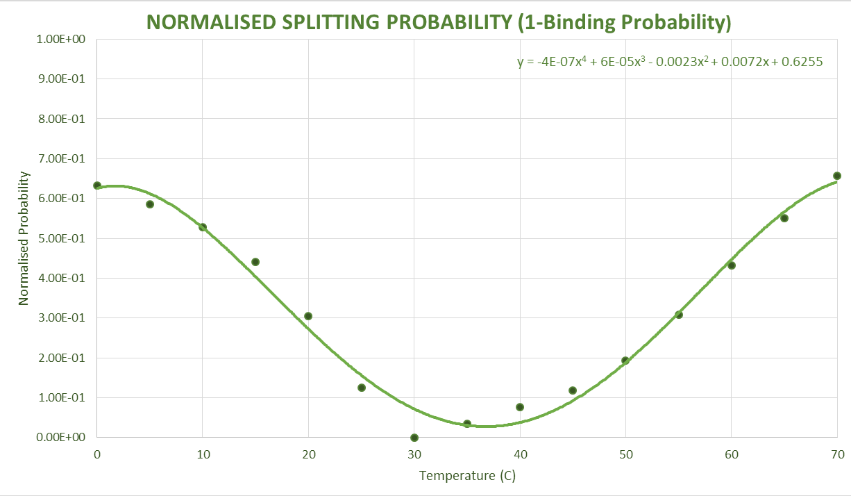
We performed in silico testing on Green et al to determine the equilibrium concentrations of the different components in our system. From this we also obtained Free energy data for the different structures; the unbound trigger, the unbound toehold and the complex of the two.
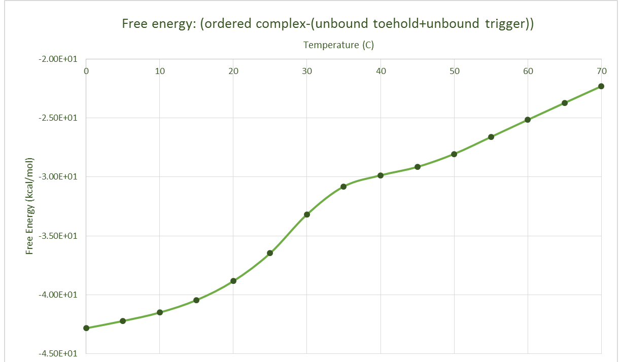
After obtaining this, we converted to an approximate normal distribution and after normalising these within the range of values, we could use the distribution as a probability distribution. This seems pointless, but it could directly be implemented into the model in the functions joiner and splitter. Shown below are these obtained probability distributions based the free energy data.
Assumptions
- Low affinity tubes
- The cell free kit components will not stick to the walls of the microcentrifuge tube.
- This assumption is made as we modelled the particles as bouncing directly of off the walls of the tube.
- These were chosen for this reason and after talking to Dr Nic Harmer, the tubes were provided by Eppendorf.
- Ribosome Stays Bound
- Once the ribosome attaches after the binding site is revealed it stays bound. It was also assumed that it makes the protein once the ribosome is bound.
- This assumption was made as a way of producing a numerical output, as it allows us to say x amount of GFP will be produced in a given time period.
- Once bound GFP is made.
- Rate of ribosome movement contains the rate of RNA, amino acid production, and all other translational steps.
- This is again needed to simplify the numerical output as above.
- Elastic collisions
- This concerns the collisions with the walls of the container, they are assumed to be elastic to simplify the maths and hence the simulation as no loss of kinetic energy is taken into account.
- Assume an excess of substrate
- This allows us to assume that translational machinery is not a limiting factor in GFP production.
- Random starting positions
- The lab team is advised to shake the tubes before an experiment to achieve this.
- Spherical particles
- The individual Toehold switches and RNA triggers are assumed to have a spherical area of influence.
- The radius of the spheres is an approximation based on the length of a base pair and the number of base pairs in the sequence.
- This was done after discussions with Peter Winlove about whether we could measure the actual size of the particles. Unfortunately we could not do this.
- Spherical binding
- As the particles are assumed to be spherical in shape we needed to assume that these would interact if the two spheres overlapped each other.
- Constant temperature
- The experiment is assumed to be carried out at a constant temperature
- Constant speed
- The particles travel in the container with a constant speed, this is made as we assume there to be no effects from gravity.
- No denaturing above a certain temperature
- (could decrease join probability at higher temperatures to correlation with decreased proportion of toeholds in correct conformation)
- Viscosity close to water [3].
- Binding distance close to the length of one Hydrogen bond [1]. Dr Nic Harmer provided us with the information to follow up on this.
Parameter Scanning
Introduction
The idea of parameter scanning is to replicate the experimental data and to develop a “harmony” between experiments and model. Using our working simulation, we proposed a multidimensional comparative scanning for the optimal input parameters and thus inference of the most desirable conditions in which to run our system. This meant running the simulation over a variety of input values in either single parameter or simultaneous multiple parameter analysis. The internal mechanics of the simulation were tuned to be as accurate as we could feasibly make them from literature research or by assumption.
The assumptions listed above are included within the model however, these created considerable uncertainty in some of our outputs, most notably the estimated translational rate of the ribosomes in our cell free kit; as well as the interaction of particles with the edge of the container.
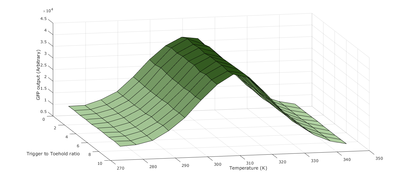
The numerical output used to quantify the performance of the system was based on the rate of production of reporter. For example, using the estimated translational rate of GFP by the ribosomes we calculated a cumulative sum of the GFP produced in one “run” of the simulation for the given parameters. Using fluorescence standards, this could be converted to an RFU value which would then allow direct comparison with lab-obtained data. However on a performance rating basis to test our different parameters, absolute GFP should be a suitable method of quantifying output.
We were also unable to validate our simulation directly using data from wet lab experiments. This meant the parameter scanning element of the simulation only produced a surface that validated the NUPACK data used to provide the probabilities of the binding and splitting mechanisms.
Parameters To Scan
First we categorised the parameters that we can vary by their logical impact and desired value, manipulability in the lab and feasibility of implementation to a field test. The main parameters to consider were:
- Temperature
- This directly influences the kinetic energy of the particles, stability of hybridisation and activity of the transcriptional and translational machinery, amongst other things.
- Concentration of plasmid DNA
- The DNA allows the transcription of the toeholds and hence will be crucial in determining the minimum concentration of plasmid required for an adequate response from the reporter to be formed.
- Concentration of RNA trigger
- The component to be detected by our toeholds, it is the limiting factor in terms of the sensitivity of our test. From conversing with vets and farmers, this must be minimised, whilst maximising the reporter output to make a robust test that works on samples containing lower concentrations of the trigger.
- Viscosity
- This is a parameter that directly impacts on the practicality of the field test version of the system. For example, increasing the viscosity would be equivalent simulating the cell free system in a gel type matrix rather than in a solution with viscosity similar to water. Conversely, decreasing the viscosity could perhaps inform on the optimal choice of solvent for the cell free system.
Scaling
Due to the vast number of particles in our real world system and the relatively low computer power available to us we took the decision to only model a subset of our system. We scaled down the number of particles by one billion this allow us to run our model at approximately 300 particles but still represent the physical system. Reducing the number by this amount let us perform parameter scanning much easier, extending the number of variables we could try and optimise.
However as we had significantly reduced the number of particles we needed to reduce the volume of the container so that the binding event would be just as frequent. The overall volume of the container also needed to be reduced by one billion. To do this we calculated the ratio of radius to height of the cylinder. This allowed the radius and height variable to be interchanged using: r = αh ; where r is the radius, h the height, and α the ratio. Using the simple volume of a cylinder formula V=Πr2h, we could calculate both the height and radius of our scaled down cylinder as we know the final volume.
Future Improvements
Toolkit
During the process we realised how much our simulation had helped the whole team, both wet and dry lab, develop an understanding for the cell free system and the parameter variables needed to make it work. We found this extremely helpful and so have decided to allow access to our matlab scripts at both stages of our simulation development. By freely allowing access to both the visual output and the parameter scanning features, future iGEM teams will have a powerful tool to both visually understand their work and numerically optimise it.
Obviously no one wants iGEM to end but unfortunately it does :( So we have made a list of those little extras that we did not get to add into the code and all those pesky bugs that we could not get out of it! Outlining these improvements allows other teams to fix them, but at least be aware of them.
Additions:
- We would like to add in a system such that at each time step the range of the random number generator is reduced, hence limiting the size of the random walk. We hope this would imitate the slowing down of the particles over time.
- Allow the user to input the variables joinprob and splitprob, the probability for joining and splitting respectively, as input arguments to the function rather than the free energy association based probabilities currently used.
- Extend the trajectory function so that it can deal with the collision at the bottom and top of our containment cylinder.
- A heatmap based display so that the previous random walk paths fade away as to not obscure the future paths.
- Use a more sophisticated method of parameter scanning based on a genetic algorithm.
Bugs:
- Trajectory function
- Trajectory correction doesn’t always place the new point in the correct quadrant, possibly due to a missing sign change in the calculations.
- Confinement and Bouncing
- Currently no code for what happens if the particle hits the top or bottom of the container. Placement at the edge of the boundary exists in the most recent construct.
- Writing of active complexes
- Occasionally, writing of the [1x3] matrix for activated complexes is written in multiple consecutive rows within points array. Thiss doesn’t effect the plotting or numerical output.
Like most iGEM projects we did not get all the data we wanted, he hope that by supplying the model along with a detailed breakdown of the lab work that other teams can use this simulation to simulate their own systems.
Summary
Due to the relatively new nature of cell free systems in synthetic biology, we built a simulation to help our understanding. We successfully developed not only a simulation but also a parameter scanning add on capable of optimising our system. We have detailed above not only the process we went through when building the model but also every intricate part of the code. We hope this is clear and that our extensive interdisciplinary approach to sourcing information relevant to the simulation, can be an example for future teams to follow. Also listed above are our proposed additions, and all of the bugs in the code that we are aware of. Our hope is that by completely documenting these as well as our method that other teams can build on our work and apply it to their own system to greater their personal knowledge and that of the iGEM community.
Matlab Scripts
A few of the many matlab scripts that we made as we went through our project. We have chosen to upload three scripts; the first is the last revision before a significant overhaul, the second is the final script, and finally the third is the script use for parameter scanning. They are linked below in both a published Matlab form, and a physical .m file stored on the iGEM servers. However in addition to both of these we have uploaded them to our GitHub Page!
Before The Change
This is the published script, and the .m file of our brownian motion simulation. This is an intermediate example of the simulation, before a significant overhaul prompted after a meeting with a computer scientist, Jonathan Fieldsend.
After The Change
Here we have the published script, the .m file and some output of our final simulation.
Parameter Scanning
Here we have the published script, the .m file and some output of parameter scanning script.
References
- Binding distance
University of Alcalá, 2014. The structure of water: hydrogen bonds. [Online] [Accessed 15 September 2015]. Available from: http://biomodel.uah.es/en/water/hbonds.html - Boundaries
Rectangleworld, 2012. Bouncing particles off a circular boundary. [Online] [Accessed 15 September 2015]. Available from: http://rectangleworld.com/blog/archives/358 - Viscosity
Promega, E. coli S30 Extract System for Circular DNA. [Online] [Accessed 15 September 2015]. Available from: https://www.promega.co.uk/~/media/files/resources/msds/l1000/l1020.pdf?la=en-gb - Ribosome speed
BSBC, Ribosome. [Online] [Accessed 15 September 2015]. Available from: http://bscb.org/learning-resources/softcell-e-learning/ribosome/ - RNA/Toehold binding time
Practically Science, 2013. Timescales, Kinetics, Rates, Half-lives in Biology. [Online] [Accessed 15 September 2015]. Available from: http://www.practicallyscience.com/timescales-kinetics-rates-half-lives-in-biology/ - 1.5ml Eppendorf dimensions
POCD Scientific, Safe-Lock Tube 1.5 mL Dimensions. [Online] [Accessed 15 September 2015]. Available from: http://www.pocdscientific.com.au/files/POCDS_pdfs/Eppendorf_Dimensions_1_5_ml_Safe_Lock_Tube.pdf - Microwell plate dimensions
Microplate Dimensions Guide, Compendium of Greiner Bio-One Microplates. [Online] [Accessed 15 September 2015]. Available from: https://www.gbo.com/fileadmin/user_upload/Downloads/Brochures/Brochures_BioScience/F073027_Microplate_Dimensions_Guide.pdf - GFP production data
iGEM, 2004. Part:BBa E0040 - parts.igem.org [Online] [Accessed 15 September 2015]. Available from: http://parts.igem.org/Part:BBa_E0040